jjjjjjjjjjjjjjj

1. CHAPTER 0
Contents
Preface v
Problems Solved in Student Solutions Manual vii
1 Matrices, Vectors, and Vector Calculus 1
2 Newtonian Mechanics—Single Particle 29
3 Oscillations 79
4 Nonlinear Oscillations and Chaos 127
5 Gravitation 149
6 Some Methods in The Calculus of Variations 165
7 Hamilton’s Principle—Lagrangian and Hamiltonian Dynamics 181
8 Central-Force Motion 233
9 Dynamics of a System of Particles 277
10 Motion in a Noninertial Reference Frame 333
11 Dynamics of Rigid Bodies 353
12 Coupled Oscillations 397
13 Continuous Systems; Waves 435
14 Special Theory of Relativity 461
iii

2. iv CONTENTS

3. CHAPTER 0
Preface
This Instructor’s Manual contains the solutions to all the end-of-chapter problems (but not the
appendices) from Classical Dynamics of Particles and Systems, Fifth Edition, by Stephen T.
Thornton and Jerry B. Marion. It is intended for use only by instructors using Classical Dynamics
as a textbook, and it is not available to students in any form. A Student Solutions Manual
containing solutions to about 25% of the end-of-chapter problems is available for sale to
students. The problem numbers of those solutions in the Student Solutions Manual are listed on
the next page.
As a result of surveys received from users, I continue to add more worked out examples in
the text and add additional problems. There are now 509 problems, a significant number over
the 4th edition.
The instructor will find a large array of problems ranging in difficulty from the simple
“plug and chug” to the type worthy of the Ph.D. qualifying examinations in classical mechanics.
A few of the problems are quite challenging. Many of them require numerical methods. Having
this solutions manual should provide a greater appreciation of what the authors intended to
accomplish by the statement of the problem in those cases where the problem statement is not
completely clear. Please inform me when either the problem statement or solutions can be
improved. Specific help is encouraged. The instructor will also be able to pick and choose
different levels of difficulty when assigning homework problems. And since students may
occasionally need hints to work some problems, this manual will allow the instructor to take a
quick peek to see how the students can be helped.
It is absolutely forbidden for the students to have access to this manual. Please do not
give students solutions from this manual. Posting these solutions on the Internet will result in
widespread distribution of the solutions and will ultimately result in the decrease of the
usefulness of the text.
The author would like to acknowledge the assistance of Tran ngoc Khanh (5th edition),
Warren Griffith (4th edition), and Brian Giambattista (3rd edition), who checked the solutions of
previous versions, went over user comments, and worked out solutions for new problems.
Without their help, this manual would not be possible. The author would appreciate receiving
reports of suggested improvements and suspected errors. Comments can be sent by email to
stt@virginia.edu, the more detailed the better.
Stephen T. Thornton
Charlottesville, Virginia
v

4. vi PREFACE

5. CHAPTER 1
Matrices, Vectors,
and Vector Calculus
1-1.
x2 = x2′
x1′
45˚
x1
45˚
x3
x3′
Axes x′ and x′ lie in the x1 x3 plane.
1 3
The transformation equations are:
x1 = x1 cos 45° − x3 cos 45°
′
x2 = x2
′
x3 = x3 cos 45° + x1 cos 45°
′
1 1
x1 =
′ x1 − x3
2 2
x2 = x2
′
1 1
x3 =
′ x1 − x3
2 2
So the transformation matrix is:
 1 1 
0 −
 2 2
 
 0 1 0 
 1 1 
 0 
 2 2 
1

6. 2 CHAPTER 1
1-2.
a)
x3
D
E
γ
β x2
O
α B
A C
x1
From this diagram, we have
OE cos α = OA
OE cos β = OB (1)
OE cos γ = OD
Taking the square of each equation in (1) and adding, we find
2 2 2 2
OE cos 2 α + cos 2 β + cos 2 γ  = OA + OB + OD
  (2)
But
2 2 2
OA + OB = OC (3)
and
2 2 2
OC + OD = OE (4)
Therefore,
2 2 2 2
OA + OB + OD = OE (5)
Thus,
cos 2 α + cos 2 β + cos 2 γ = 1 (6)
b)
x3
D
E
D′
E′
θ B B′ x2
O
A A′ C C′
x1
First, we have the following trigonometric relation:
OE + OE′ − 2OE OE′ cos θ = EE′
2 2 2
(7)

7. MATRICES, VECTORS, AND VECTOR CALCULUS 3
But,
2 2 2
     
EE′ = OB′ − OB  + OA′ − OA  + OD′ − OD 
2
     
2 2
   
= OE′ cos β ′ − OE cos β  + OE′ cos α ′ − OE cos α 
   
2
 
+ OE′ cos γ ′ − OE cos γ  (8)
 
or,
EE′ = OE′ cos 2 α ′ + cos 2 β ′ + cos 2 γ ′  + OE  cos 2 α + cos 2 β + cos 2 γ 
2 2 2
   
− 2OE′ OE cos α cos α ′ + cos β cos β ′ + cos γ cos γ ′ 
 
= OE′ 2 + OE2 − 2OE OE′ cos α cos α ′ + cos β cos β ′ + cos γ cos γ ′ 
  (9)
Comparing (9) with (7), we find
cos θ = cos α cos α ′ + cos β cos β ′ + cos γ cos γ ′ (10)
1-3.
x3
A e3 e2′
e3
O x2 e2
e1
e2 e1′
x1 e1 e3′
Denote the original axes by x1 , x2 , x3 , and the corresponding unit vectors by e1 , e2 , e3 . Denote
1 2 3 ′ ′ ′
the new axes by x′ , x′ , x′ and the corresponding unit vectors by e1 , e2 , e3 . The effect of the
rotation is e1 → e3 , e2 → e1 , e3 → e2 . Therefore, the transformation matrix is written as:
′ ′ ′
 cos ( e1 , e1 ) cos ( e1 , e2 ) cos ( e1 , e3 )  0 1 0 
′ ′ ′
 
λ = cos ( e′ , e1 ) cos ( e′ , e2 ) cos ( e′ , e3 )  = 0 0 1 
2 2 2  
  1 0 0 
 cos ( e′ , e1 ) cos ( e′ , e2 ) cos ( e′ , e3 )  
3 3 3 
1-4.
a) Let C = AB where A, B, and C are matrices. Then,
Cij = ∑ Aik Bkj (1)
k
(C )
t
ij
= C ji = ∑ Ajk Bki = ∑ Bki Ajk
k k

8. 4 CHAPTER 1
( )
Identifying Bki = Bt ik
( )
and Ajk = At kj
,
(C ) = ∑ (B ) ( A )
t
ij
t
ik
t
kj
(2)
k
or,
C t = ( AB) = Bt At
t
(3)
b) To show that ( AB) = B−1 A−1 ,
−1
( AB) B−1 A−1 = I = ( B−1 A−1 ) AB (4)
That is,
( AB) B−1 A−1 = AIA−1 = AA−1 = I (5)
(B −1
)
A−1 ( AB) = B−1 IB = B−1B = I (6)
1-5. Take λ to be a two-dimensional matrix:
λ11 λ12
λ = = λ11λ 22 − λ12 λ 21 (1)
λ 21 λ 22
Then,
λ = λ11λ 22 − 2λ11λ 22 λ12 λ 21 + λ12 λ 21 + ( λ11λ 21 + λ12 λ 22 ) − ( λ11λ 21 + λ12λ 22 )
2 2 2 2 2 2 2 2 2 2 2 2 2
(2 2
) 2 2 2
( 2 2
) (
= λ 22 λ11 + λ12 + λ 21 λ11 + λ12 − λ11λ 21 + 2λ11λ 22λ12 λ 21 + λ12λ 22
2 2 2
)
(2 2
)(
2 2
)
= λ11 + λ12 λ 22 + λ 21 − ( λ11λ 21 + λ12 λ 22 )
2
(2)
But since λ is an orthogonal transformation matrix, ∑λ λ ij kj = δ ik .
j
Thus,
λ11 + λ12 = λ 21 + λ 22 = 1
2 2 2 2
(3)
λ11λ 21 + λ12 λ 22 = 0
Therefore, (2) becomes
λ =1
2
(4)
1-6. The lengths of line segments in the x j and x ′ systems are
j
L= ∑x 2
j ; L′ = ∑ x′ i
2
(1)
j i

9. MATRICES, VECTORS, AND VECTOR CALCULUS 5
If L = L ′ , then
∑ x = ∑ x′ 2
j i
2
(2)
j i
The transformation is
xi′ = ∑ λ ij x j (3)
j
Then,
  
∑ x = ∑∑λ
2

j ik xk   ∑ λ i x 
 
j i k
(4)
 
= ∑ xk x  ∑ λik λ i 
k,  i 
But this can be true only if
∑λ ik λi = δ k (5)
i
which is the desired result.
1-7.
x3
(0,0,1) (0,1,1)
(1,1,1)
(1,0,1)
x2
(0,0,0) (0,1,0)
(1,0,0) (1,1,0)
x1
There are 4 diagonals:
D1 , from (0,0,0) to (1,1,1), so (1,1,1) – (0,0,0) = (1,1,1) = D1 ;
D 2 , from (1,0,0) to (0,1,1), so (0,1,1) – (1,0,0) = (–1,1,1) = D 2 ;
D 3 , from (0,0,1) to (1,1,0), so (1,1,0) – (0,0,1) = (1,1,–1) = D 3 ; and
D 4 , from (0,1,0) to (1,0,1), so (1,0,1) – (0,1,0) = (1,–1,1) = D 4 .
The magnitudes of the diagonal vectors are
D1 = D 2 = D 3 = D 4 = 3
The angle between any two of these diagonal vectors is, for example,
D1 ⋅ D 2 (1,1,1) ⋅ ( −1,1,1) 1
= cos θ = =
D1 D 2 3 3

10. 6 CHAPTER 1
so that
 1
θ = cos−1   = 70.5°
 3
Similarly,
D1 ⋅ D 3 D ⋅D D ⋅D D ⋅D D ⋅D 1
= 1 4 = 2 3 = 2 4 = 3 4 =±
D1 D 3 D1 D 4 D2 D3 D2 D 4 D3 D 4 3
1-8. Let θ be the angle between A and r. Then, A ⋅ r = A2 can be written as
Ar cos θ = A2
or,
r cos θ = A (1)
This implies
π
QPO = (2)
2
Therefore, the end point of r must be on a plane perpendicular to A and passing through P.
1-9. A = i + 2j − k B = −2i + 3j + k
a) A − B = 3i − j − 2k
12
A − B = ( 3) + ( −1) + (−2)2 
2 2
 
A − B = 14
b)
B
θ
A
component of B along A
The length of the component of B along A is B cos θ.
A ⋅ B = AB cos θ
A ⋅ B −2 + 6 − 1 3 6
B cos θ = = = or
A 6 6 2
The direction is, of course, along A. A unit vector in the A direction is
1
( i + 2j − k )
6

11. MATRICES, VECTORS, AND VECTOR CALCULUS 7
So the component of B along A is
1
2
( i + 2j − k )
A⋅B 3 3 3
c) cos θ = = = ; θ = cos −1
AB 6 14 2 7 2 7
θ 71°
i j k
2 −1 1 −1 1 2
d) A × B = 1 2 −1 = i −j +k
3 1 −2 1 −2 3
−2 3 1
A × B = 5i + j + 7 k
e) A − B = 3i − j − 2k A + B = −i + 5j
i j k
( A − B ) × ( A + B ) = 3 −1 − 2
−1 5 0
( A − B) × ( A + B) = 10i + 2j + 14k
1-10. r = 2b sin ω t i + b cos ω t j
v = r = 2bω cos ω t i − bω sin ω t j
a)
a = v = −2bω 2 sin ω t i − bω 2 cos ω t j = −ω 2 r
12
speed = v =  4b 2ω 2 cos 2 ω t + b 2ω 2 sin 2 ω t 
 
12
= bω  4 cos 2 ω t + sin 2 ω t 
 
12
speed = bω  3 cos 2 ω t + 1
 
b) At t = π 2ω , sin ω t = 1 , cos ω t = 0
So, at this time, v = − bω j , a = −2bω 2 i
So, θ 90°

12. 8 CHAPTER 1
1-11.
a) Since ( A × B) i = ∑ ε ijk Aj Bk , we have
jk
(A × B) ⋅ C = ∑∑ ε ijk Aj Bk Ci
i j,k
= C1 ( A2 B3 − A3 B2 ) − C2 ( A1B3 − A3 B1 ) + C3 ( A1B2 − A2 B1 ) (1)
C1 C2 C3 A1 A2 A3 A1 A2 A3
= A1 A2 A3 = − C1 C2 C3 = B1 B2 B3 = A ⋅ ( B × C )
B1 B2 B3 B1 B2 B3 C1 C2 C3
We can also write
C1 C2 C3 B1 B2 B3
(A × B) ⋅ C = − B1 B2 B3 = C1 C2 C3 = B ⋅ ( C × A ) (2)
A1 A2 A3 A1 A2 A3
We notice from this result that an even number of permutations leaves the determinant
unchanged.
b) Consider vectors A and B in the plane defined by e1 , e2 . Since the figure defined by A, B,
C is a parallelepiped, A × B = e3 × area of the base, but e3 ⋅ C = altitude of the parallelepiped.
Then,
C ⋅ ( A × B) = ( C ⋅ e3 ) × area of the base
= altitude × area of the base
= volume of the parallelepiped
1-12.
O
c
C
a h a–c
b c–b
A
b–a
B
The distance h from the origin O to the plane defined by A, B, C is

13. MATRICES, VECTORS, AND VECTOR CALCULUS 9
a ⋅ ( b − a ) × ( c − b)
h=
( b − a ) × ( c − b)
a ⋅ ( b × c − a × c + a × b)
=
b×c−a×c+a×b
a⋅b× c
= (1)
a×b+b×c+c×a
The area of the triangle ABC is:
1 1 1
A= ( b − a ) × ( c − b) = ( a − c ) × ( b − a ) = ( c − b ) × ( a − c ) (2)
2 2 2
1-13. Using the Eq. (1.82) in the text, we have
A × B = A × ( A × X ) = ( X ⋅ A ) A − ( A ⋅ A ) X = φ A − A2 X
from which
( B × A ) + φA
X=
A2
1-14.
 1 2 −1  2 1 0   1 −2 1 
    
a) AB =  0 3 1  0 −1 2  =  1 −2 9 
 2 0 1   1 1 3  5 3 3
    
Expand by the first row.
−2 9 1 9 1 −2
AB = 1 +2 +1
3 3 5 3 5 3
AB = −104
 1 2 −1  2 1   9 7 
    
b) AC = 0 3 1   4 3  = 13 9 
2 0 1   1 0  5 2
    
 9 7
 
AC = 13 9 
 5 2
 

14. 10 CHAPTER 1
 1 2 −1  8 5
  
c) ABC = A ( BC ) = 0 3 1   −2 −3 
2 0 1   9 4 
  
 −5 −5 
 
ABC =  3 −5 
 25 14 
 
d) AB − Bt At = ?
 1 −2 1 
 
AB =  1 −2 9  (from part a )
 5 3 3
 
 2 0 1  1 0 2  1 1 5
    
B A =  1 −1 1   2 3 0  =  −2 −2 3 
t t
 0 2 3   −1 1 1   1 9 3 
    
 0 −3 −4 
 
AB − B A =  3 0
t t
6
 4 −6 0 
 
1-15. If A is an orthogonal matrix, then
At A = 1
1 0 0 1 0 0  1 0 0
    
0 a a  0 a − a  = 0 1 0 
0 − a a  0 a a  0 0 1
    
1 0 0  1 0 0
   
0 2a
2
0  = 0 1 0 
0 0
 2a 2  0 0 1 
  
1
a=
2

15. MATRICES, VECTORS, AND VECTOR CALCULUS 11
1-16.
x3 P
r
θ a r
θ a
x2
x1 r cos θ
r ⋅ a = constant
ra cos θ = constant
It is given that a is constant, so we know that
r cos θ = constant
But r cos θ is the magnitude of the component of r along a.
The set of vectors that satisfy r ⋅ a = constant all have the same component along a; however, the
component perpendicular to a is arbitrary.
Thus the surface represented by r ⋅ a = constant
is a plane perpendicular to a.
1-17.
a
B C
θ
c b
A
Consider the triangle a, b, c which is formed by the vectors A, B, C. Since
C= A−B
C = ( A − B) ⋅ ( A − B)
2
(1)
= A 2 − 2A ⋅ B + B 2
or,
C = A2 + B2 − 2 AB cos θ
2
(2)
which is the cosine law of plane trigonometry.
1-18. Consider the triangle a, b, c which is formed by the vectors A, B, C.
a
α C
B
γ β
c b
A

16. 12 CHAPTER 1
C=A−B (1)
so that
C × B = ( A − B) × B (2)
but the left-hand side and the right-hand side of (2) are written as:
C × B = BC sin α e3 (3)
and
( A − B) × B = A × B − B × B = A × B = AB sin γ e3 (4)
where e3 is the unit vector perpendicular to the triangle abc. Therefore,
BC sin α = AB sin γ (5)
or,
C A
=
sin γ sin α
Similarly,
C A B
= = (6)
sin γ sin α sin β
which is the sine law of plane trigonometry.
1-19.
x2
a2 a
b2 b
α
β
x1
a1 b1
a) We begin by noting that
a − b = a 2 + b 2 − 2ab cos (α − β )
2
(1)
We can also write that
a − b = ( a1 − b1 ) + ( a2 − b2 )
2 2 2
= ( a cos α − b cos β ) + ( a sin α − b sin β )
2 2
( ) ( )
= a 2 sin 2 α + cos 2 α + b 2 sin 2 β + cos 2 β − 2 ab ( cos α cos β + sin α sin β )
= a 2 + b 2 − 2ab ( cos α cos β + sin α sin β ) (2)

17. MATRICES, VECTORS, AND VECTOR CALCULUS 13
Thus, comparing (1) and (2), we conclude that
cos (α − β ) = cos α cos β + sin α sin β (3)
b) Using (3), we can find sin (α − β ) :
sin (α − β ) = 1 − cos 2 (α − β )
= 1 − cos 2 α cos 2 β − sin 2 α sin 2 β − 2cos α sin α cos β sin β
( ) (
= 1 − cos 2 α 1 − sin 2 β − sin 2 α 1 − cos 2 β − 2cos α sin α cos β sin β )
= sin 2 α cos 2 β − 2sin α sin β cos α cos β + cos 2 α sin 2 β
= ( sin α cos β − cos α sin β )2 (4)
so that
sin (α − β ) = sin α cos β − cos α sin β (5)
1-20.
a) Consider the following two cases:
When i ≠ j δ ij = 0 but ε ijk ≠ 0 .
When i = j δ ij ≠ 0 but ε ijk = 0 .
Therefore,
∑ε ijk δ ij = 0 (1)
ij
b) We proceed in the following way:
When j = k, ε ijk = ε ijj = 0 .
Terms such as ε j11 ε 11 = 0 . Then,
∑ε ijk ε jk = ε i12 ε 12 + ε i13 ε 13 + ε i 21 ε 21 + ε i 31 ε 31 + ε i 32 ε 32 + ε i 23 ε 23
jk
Now, suppose i = = 1 , then,
∑= ε 123 ε 123 + ε 132 ε 132 = 1 + 1 = 2
jk

18. 14 CHAPTER 1
for i = = 2 , ∑= ε 213 ε 213 + ε 231 ε 231 = 1 + 1 = 2 . For i = = 3 , ∑= ε 312 ε 312 + ε 321 ε 321 = 2 . But i = 1,
jk jk
= 2 gives ∑ = 0 . Likewise for i = 2, = 1 ; i = 1, = 3 ; i = 3, = 1 ; i = 2, = 3 ; i = 3, = 2.
jk
Therefore,
∑ε ijk ε jk = 2δ i (2)
j,k
c) ∑ε ijk ε ijk = ε 123 ε 123 + ε 312 ε 312 + ε 321 ε 321 + ε 132 ε 132 + ε 213 ε 213 + ε 231 ε 231
ijk
= 1 ⋅ 1 + 1 ⋅ 1 + ( −1) ⋅ ( −1) + ( −1) ⋅ ( −1) + ( −1) ⋅ ( −1) + (1) ⋅ (1)
or,
∑ε ijk ε ijk = 6 (3)
ijk
1-21. ( A × B)i = ∑ ε ijk Aj Bk (1)
jk
( A × B) ⋅ C = ∑ ∑ε ijk Aj Bk Ci (2)
i jk
By an even permutation, we find
ABC = ∑ ε ijk Ai Bj Ck (3)
ijk
1-22. To evaluate ∑ε ijk ε mk we consider the following cases:
k
a) i= j: ∑ε ijk ε mk = ∑ ε iik ε mk = 0 for all i , , m
k k
b) i= : ∑ε ijk ε mk = ∑ ε ijk ε imk = 1 for j = m and k ≠ i , j
k k
= 0 for j ≠ m
c) i = m: ∑ε ijk ε mk = ∑ ε ijk ε ik = 0 for j ≠
k k
= −1 for j = and k ≠ i , j
d) j= : ∑ε ijk ε mk = ∑ ε ijk ε jmk = 0 for m ≠ i
k k
= −1 for m = i and k ≠ i , j

19. MATRICES, VECTORS, AND VECTOR CALCULUS 15
e) j = m: ∑ε ijk ε mk = ∑ ε ijk ε jk = 0 for i ≠
k k
= 1 for i = and k ≠ i , j
f) = m: ∑ε ijk ε mk = ∑ ε ijk ε k = 0 for all i , j , k
k k
g) i ≠ or m : This implies that i = k or i = j or m = k.
Then, ∑ε ijk ε mk = 0 for all i , j , , m
k
h) j ≠ or m : ∑ε ijk ε mk = 0 for all i , j , , m
k
Now, consider δ i δ jm − δ im δ j and examine it under the same conditions. If this quantity
behaves in the same way as the sum above, we have verified the equation
∑ε ijk ε mk = δ i δ jm − δ im δ j
k
a) i = j : δ i δ im − δ im δ i = 0 for all i , , m
b) i = : δ ii δ jm − δ im δ ji = 1 if j = m, i ≠ j , m
= 0 if j ≠ m
c) i = m : δ i δ ji − δ ii δ j = −1 if j = , i ≠ j ,
= 0 if j ≠
d) j = : δi δ m − δ im δ = −1 if i = m, i ≠
= 0 if i ≠ m
e) j = m : δ i δ mm − δ im δ m = 1 if i = , m ≠
= 0 if i ≠
f) = m : δ i δ j − δ il δ j = 0 for all i , j ,
g) i ≠ , m : δ i δ jm − δ im δ j = 0 for all i , j , , m
h) j ≠ , m : δ i δ jm − δ im δ i = 0 for all i , j , , m
Therefore,
∑ε ijk ε mk = δ i δ jm − δ im δ j (1)
k
Using this result we can prove that
A × ( B × C ) = ( A ⋅ C ) B − ( A ⋅ B) C

20. 16 CHAPTER 1
First ( B × C ) i = ∑ ε ijk Bj Ck . Then,
jk
[ A × (B × C) ] = ∑ ε mn Am ( B × C ) n = ∑ ε mn Am ∑ ε njk BjCk
mn mn jk
= ∑ε mn ε njk Am Bj Ck = ∑ε mn ε jkn Am Bj Ck
jkmn jkmn
 
= ∑  ∑ ε lmn ε jkn  Am Bj Ck
jkm  n 
( )
= ∑ δ jlδ km − δ k δ jm Am Bj Ck
jkm
   
= ∑ Am B Cm − ∑ Am BmC = B  ∑ AmCm  − C  ∑ Am Bm 
m m  m   m 
= ( A ⋅ C ) B − ( A ⋅ B) C
Therefore,
A × ( B × C ) = ( A ⋅ C ) B − ( A ⋅ B) C (2)
1-23. Write
( A × B) j = ∑ ε j m A Bm
m
( C × D) k = ∑ ε krs Cr Ds
rs
Then,

21. MATRICES, VECTORS, AND VECTOR CALCULUS 17
  
[ ( A × B) × (C × D)]i = ∑ ε ijk  ∑ ε j m A Bm   ∑ ε krs Cr Ds 
  
jk m rs
= ∑ε ijk ε j m ε krs A BmCr Ds
jk mrs
 
= ∑ε j m  ∑ ε ijk ε rsk  A BmCr Ds
 k 
j mrs
= ∑ ε (δ j m ir )
δ js − δ is δ jr A BmCr Ds
j mrs
(
= ∑ ε j m A BmCi Dj − A Bm Di C j
j m
)
   
=  ∑ ε j m Dj A Bm  Ci −  ∑ ε j m C j A Bm  Di
jm  jm 
= (ABD)Ci − (ABC)Di
Therefore,
[( A × B) × (C × D) ] = (ABD)C − (ABC)D
1-24. Expanding the triple vector product, we have
e × ( A × e) = A ( e ⋅ e) − e ( A ⋅ e) (1)
But,
A ( e ⋅ e) = A (2)
Thus,
A = e ( A ⋅ e) + e × ( A × e) (3)
e(A · e) is the component of A in the e direction, while e × (A × e) is the component of A
perpendicular to e.

22. 18 CHAPTER 1
1-25.
er
eφ
θ
φ
eθ
The unit vectors in spherical coordinates are expressed in terms of rectangular coordinates by
eθ = ( cos θ cos φ , cos θ sin φ , − sin θ ) 


eφ = ( − sin φ , cos φ , 0 )  (1)

er = ( sin θ cos φ , sin θ sin φ , cos θ )  
Thus,
(
eθ = −φ cos θ sin φ − θ sin θ cos φ , φ cos θ cos φ − θ sin θ sin φ , − θ cos θ )
= −θ er + φ cos θ eφ (2)
Similarly,
(
eφ = −φ cos φ , − φ sin φ , 0 )
= −φ cos θ eθ − φ sin θ er (3)
er = φ sin θ eφ + θ eθ (4)
Now, let any position vector be x. Then,
x = rer (5)
( )
x = rer + rer = r φ sin θ eφ + θ eθ + rer
= rφ sin θ eφ + rθ eθ + rer (6)
( ) ( )
x = rφ sin θ + rθφ cos θ + rφ sin θ eφ + rφ sin θ eφ + rθ + rθ eθ + rθ eθ + rer + rer
( ) (
= 2rφ sin θ + 2rθφ cos θ + rφ sin θ eφ + r − rφ 2 sin 2 θ − rθ 2 er )
(
+ 2rθ + rθ − rφ 2 sin θ cos θ eθ ) (7)
or,

23. MATRICES, VECTORS, AND VECTOR CALCULUS 19
 
1 d 2
x = a =  r − rθ 2 − rφ 2 sin 2 θ  er + 
 r dt
( ) 
r θ − rφ 2 sin θ cos θ  eθ

(8)
 1 
+
d 2
(
r φ sin 2 θ  eφ )
 r sin θ dt 
1-26. When a particle moves along the curve
r = k (1 + cos θ ) (1)
we have
r = − kθ sin θ 
 (2)

r = − k θ cos θ + θ sin θ  

2

Now, the velocity vector in polar coordinates is [see Eq. (1.97)]
v = rer + rθ eθ (3)
so that
v 2 = v = r 2 + r 2θ 2
2
( )
= k 2θ 2 sin 2 θ + k 2 1 + 2 cos θ + cos 2 θ θ 2
= k 2θ 2 2 + 2 cos θ 
  (4)
and v 2 is, by hypothesis, constant. Therefore,
v2
θ= (5)
2k (1 + cos θ )
2
Using (1), we find
v
θ= (6)
2kr
Differentiating (5) and using the expression for r , we obtain
v 2 sin θ v 2 sin θ
θ= = 2 (7)
4 k (1 + cos θ )
2
4r 2
The acceleration vector is [see Eq. (1.98)]
( )
a = r − rθ 2 er + rθ + 2rθ eθ( ) (8)
so that

24. 20 CHAPTER 1
a ⋅ er = r − rθ 2
( )
= − k θ 2 cos θ + θ sin θ − k (1 + cos θ ) θ 2
 θ 2 sin 2 θ 
= − k θ 2 cos θ + + (1 + cos θ ) θ 2 

 2 (1 + cos θ ) 

 1 − cos 2 θ 
= − kθ 2  2 cos θ + + 1

 2 (1 + cos θ )  
3
= − kθ 2 (1 + cos θ ) (9)
2
or,
3 v2
a ⋅ er = − (10)
4 k
In a similar way, we find
3 v 2 sin θ
a ⋅ eθ = − (11)
4 k 1 + cos θ
From (10) and (11), we have
a = ( a ⋅ er ) 2 + ( a ⋅ eθ ) 2 (12)
or,
3 v2 2
a = (13)
4 k 1 + cos θ
1-27. Since
r × (v × r) = (r ⋅ r) v − (r ⋅ v) r
we have
d d
dt
[ r × ( v × r ) ] = dt [ ( r ⋅ r ) v − ( r ⋅ v ) r ]
= (r ⋅ r) a + 2 (r ⋅ v) v − (r ⋅ v) v − ( v ⋅ v) r − (r ⋅ a) r
(
= r 2a + ( r ⋅ v ) v − r v2 + r ⋅ a ) (1)
Thus,
d
dt
(
[ r × ( v × r )] = r 2a + ( r ⋅ v ) v − r r ⋅ a + v 2 ) (2)

25. MATRICES, VECTORS, AND VECTOR CALCULUS 21
∂
1-28. grad ( ln r ) = ∑ ( ln r ) ei (1)
i ∂x i
where
r = ∑x 2
i (2)
i
Therefore,
∂ 1 xi
( ln r ) = r
∂x i ∑x 2
i
i
xi
= 2
(3)
r
so that
1  
grad ( ln r ) = 2 ∑ i i
xe (4)
r  i 
or,
r
grad ( ln r ) = (5)
r2
1-29. Let r 2 = 9 describe the surface S1 and x + y + z 2 = 1 describe the surface S2 . The angle θ
between S1 and S2 at the point (2,–2,1) is the angle between the normals to these surfaces at the
point. The normal to S1 is
( )
grad ( S1 ) = grad r 2 − 9 = grad x 2 + y 2 + z 2 − 9 ( )
= ( 2xe1 + 2 ye2 + 2ze3 ) x = 2, y = 2, z = 1 (1)
= 4e1 − 4e2 + 2e3
In S2 , the normal is:
(
grad ( S2 ) = grad x + y + z 2 − 1 )
= ( e1 + e2 + 2ze3 ) x = 2, y =−2, z = 1 (2)
= e1 + e2 + 2e3
Therefore,

26. 22 CHAPTER 1
grad ( S1 ) ⋅ grad ( S2 )
cos θ =
grad ( S1 ) grad ( S2 )
=
( 4e1 − 4e2 + 2e3 ) ⋅ (e1 + e2 + 2e3 ) (3)
6 6
or,
4
cos θ = (4)
6 6
from which
6
θ = cos −1 = 74.2° (5)
9
3
∂ ( φψ )  ∂ψ ∂ φ 
1-30. grad ( φψ ) = ∑ ei = ∑ ei φ + ψ
i =1 ∂x i i  ∂x i ∂x i 
∂ψ ∂φ
= ∑ ei φ + ∑ ei ψ
i ∂x i i ∂x i
Thus,
grad ( φψ ) = φ grad ψ + ψ grad φ
1-31.
a)
n
∂   
12
∂rn
3
grad r = ∑ ei
n
= ∑ ei  ∑ xj  
2
∂x i ∂x i   j  
i =1
 
n
−1
n 2
= ∑ ei 2 xi  ∑ x 2 
j
i 2 j 
n
−1
 2
= ∑ ei x i n  ∑ x 2 
j
i  j 
= ∑ ei x i n r ( n − 2) (1)
i
Therefore,
grad r n = nr ( n − 2) r (2)

27. MATRICES, VECTORS, AND VECTOR CALCULUS 23
b)
3
∂f ( r ) 3 ∂ f ( r ) ∂ r
grad f ( r ) = ∑ ei = ∑ ei
i =1 ∂x i i =1 ∂ r ∂x i
12
∂   ∂f ( r )
= ∑ ei  ∑ xj 
2
i ∂x i  j  ∂r
−1 2
  ∂f ( r )
= ∑ ei xi  ∑ x 2 
∂r
j
i  j 
x i ∂f
= ∑ ei (3)
i r dr
Therefore,
r ∂f ( r )
grad f ( r ) = (4)
r ∂r
c)
∂2    
12
∂ 2 ln r
∇ ( ln r ) = ∑
2
= ∑ 2  ln  ∑ x j  
2
∂xi2 ∂x i   j  
i
 
−1 2
1   
 ⋅ 2 xi  ∑ x 2 
j

∂ 2  j  
=∑  
i ∂x i 
12
  
 ∑ xj 
2
 

  j  

−1
∂    
=∑  xi  ∑ x 2  
i ∂x i
j
  j  
 
−2 −1
  ∂x  
= ∑ ( − xi )( 2xi )  ∑ x 2  + ∑ i  ∑ x2 
i ∂x i  j
j j
i  j  
(
= ∑ −2x 2 r 2
i
j )( ) −2 1
+ 3 2 
r 
2r 2 3 1
=− 4
+ 2 = 2 (5)
r r r
or,
1
∇ 2 ( ln r ) = (6)
r2

28. 24 CHAPTER 1
1-32. Note that the integrand is a perfect differential:
d d
2ar ⋅ r + 2br ⋅ r = a (r ⋅ r) + b (r ⋅ r) (1)
dt dt
Clearly,
∫ ( 2ar ⋅ r + 2br ⋅ r ) dt = ar + br 2 + const.
2
(2)
1-33. Since
d  r  rr − rr r rr
= = − 2 (1)
dt  r 
  r2 r r
we have
 r rr  d r 
∫  r − r 2  dt = ∫ dt  r  dt
    (2)
from which
 r rr  r
∫  r − r 2  dt = r + C
 
(3)
where C is the integration constant (a vector).
1-34. First, we note that
d
dt
( )
A×A =A×A+A×A (1)
But the first term on the right-hand side vanishes. Thus,
∫ ( A × A) dt = ∫ dt ( A × A) dt
d
(2)
so that
∫ ( A × A) dt = A × A + C (3)
where C is a constant vector.

29. MATRICES, VECTORS, AND VECTOR CALCULUS 25
1-35.
y
x
z
We compute the volume of the intersection of the two cylinders by dividing the intersection
volume into two parts. Part of the common volume is that of one of the cylinders, for example,
the one along the y axis, between y = –a and y = a:
( )
V1 = 2 π a 2 a = 2π a 3 (1)
The rest of the common volume is formed by 8 equal parts from the other cylinder (the one
along the x-axis). One of these parts extends from x = 0 to x = a, y = 0 to y = a 2 − x 2 , z = a to
z = a 2 − x 2 . The complementary volume is then
a a2 − x 2 a2 − x 2
V2 = 8 ∫ dx ∫ dy ∫ dz
0 0 a
= 8 ∫ dx a 2 − x 2  a 2 − x 2 − a 
a
0  
a
 x 3 a3 x
= 8  a2 x − − sin −1 
 3 2 a 0
16 3
= a − 2π a 3 (2)
3
Then, from (1) and (2):
16 a 3
V = V1 + V2 = (3)
3

30. 26 CHAPTER 1
1-36.
z
d
y
x c2 = x2 + y2
The form of the integral suggests the use of the divergence theorem.
∫ S
A ⋅ da = ∫ ∇ ⋅ A dv
V
(1)
Since ∇ ⋅ A = 1 , we only need to evaluate the total volume. Our cylinder has radius c and height
d, and so the answer is
∫ V
dv = π c 2 d (2)
1-37.
z
R
y
x
To do the integral directly, note that A = R3er , on the surface, and that da = daer .
∫ S
A ⋅ da = R 3 ∫ S
da = R3 × 4π R 2 = 4π R 5 (1)
To use the divergence theorem, we need to calculate ∇ ⋅ A . This is best done in spherical
coordinates, where A = r 3er . Using Appendix F, we see that
1 ∂ 2
∇⋅A =
r 2 ∂r
(
r A r = 5r 2 ) (2)
Therefore,
( )
π 2π R
∫ V
∇ ⋅ A dv = ∫ sin θ dθ ∫
0 0
dφ ∫ r 2 5r 2 dr = 4π R5
0
(3)
Alternatively, one may simply set dv = 4π r 2 dr in this case.

31. MATRICES, VECTORS, AND VECTOR CALCULUS 27
1-38.
z z = 1 – x2 – y2
y
C
x2 + y2 = 1
x
By Stoke’s theorem, we have
∫ (∇ × A) ⋅ da = ∫
S C
A ⋅ ds (1)
The curve C that encloses our surface S is the unit circle that lies in the xy plane. Since the
element of area on the surface da is chosen to be outward from the origin, the curve is directed
counterclockwise, as required by the right-hand rule. Now change to polar coordinates, so that
we have ds = dθ eθ and A = sin θ i + cos θ k on the curve. Since eθ ⋅ i = − sin θ and eθ ⋅ k = 0 , we
have
( − sin θ ) dθ = −π
2π
∫ A ⋅ ds = ∫ 2
(2)
C 0
1-39.
a) Let’s denote A = (1,0,0); B = (0,2,0); C = (0,0,3). Then AB = (−1, 2, 0) ; AC = (−1, 0, 3) ; and
AB × AC = (6, 3, 2) . Any vector perpendicular to plane (ABC) must be parallel to AB × AC , so
the unit vector perpendicular to plane (ABC) is n = (6 7 , 3 7 , 2 7 )
b) Let’s denote D = (1,1,1) and H = (x,y,z) be the point on plane (ABC) closest to H. Then
DH = ( x − 1, y − 1, z − 1) is parallel to n given in a); this means
x−1 6 x −1 6
= =2 and = =3
y−1 3 z−1 2
Further, AH = ( x − 1, y , z) is perpendicular to n so one has 6( x − 1) + 3 y + 2 z = 0 .
Solving these 3 equations one finds
5
H = ( x , y , z) = (19 49 , 34 49 , 39 49) and DH =
7
1-40.
a) At the top of the hill, z is maximum;
∂z ∂z
0= = 2 y − 6 x − 18 and 0= = 2 x − 8 y + 28
∂x ∂y

32. 28 CHAPTER 1
so x = –2 ; y = 3, and the hill’s height is max[z]= 72 m. Actually, this is the max value of z,
because the given equation of z implies that, for each given value of x (or y), z describes an
upside down parabola in term of y ( or x) variable.
b) At point A: x = y = 1, z = 13. At this point, two of the tangent vectors to the surface of the
hill are
∂z ∂z
t1 = (1, 0, ) = (1, 0, −8) and t2 = (0,1, ) = (0,1, 22)
∂x (1,1) ∂y (1,1)
Evidently t1 × t2 = (8, −22,1) is perpendicular to the hill surface, and the angle θ between this
and Oz axis is
(0, 0,1) ⋅ (8, −22,1) 1
cos θ = = so θ = 87.55 degrees.
8 + 22 + 1
2 2 2 23.43
c) Suppose that in the α direction ( with respect to W-E axis), at point A = (1,1,13) the hill is
steepest. Evidently, dy = (tan α )dx and
dz = 2xdy + 2 ydx − 6 xdx − 8 ydy − 18 dx + 28 dy = 22(tan α − 1)dx
then
dx 2 + dy 2 dx cos α −1
tan β = = =
dz 22(tan α − 1)dx 22 2 cos (α + 45)
The hill is steepest when tan β is minimum, and this happens when α = –45 degrees with
respect to W-E axis. (note that α = 135 does not give a physical answer).
1-41.
A ⋅ B = 2a( a − 1)
then A ⋅ B = 0 if only a = 1 or a = 0.

33. CHAPTER 2
Newtonian Mechanics—
Single Particle
2-1. The basic equation is
F = mi xi (1)
a) F ( xi , t ) = f ( xi ) g ( t ) = mi xi : Not integrable (2)
b) F ( xi , t ) = f ( xi ) g ( t ) = mi xi
dxi
mi = f ( xi ) g ( t )
dt
dxi g (t)
= dt : Integrable (3)
f ( xi ) mi
c) F ( xi , xi ) = f ( xi ) g ( xi ) = mi xi : Not integrable (4)
2-2. Using spherical coordinates, we can write the force applied to the particle as
F = Fr er + Fθ eθ + Fφ eφ (1)
But since the particle is constrained to move on the surface of a sphere, there must exist a
reaction force − Fr er that acts on the particle. Therefore, the total force acting on the particle is
Ftotal = Fθ eθ + Fφ eφ = mr (2)
The position vector of the particle is
r = Re r (3)
where R is the radius of the sphere and is constant. The acceleration of the particle is
a = r = Re r (4)
29

34. 30 CHAPTER 2
We must now express er in terms of er , eθ , and eφ . Because the unit vectors in rectangular
coordinates, e1 , e2 , e3 , do not change with time, it is convenient to make the calculation in
terms of these quantities. Using Fig. F-3, Appendix F, we see that
er = e1 sin θ cos φ + e2 sin θ sin φ + e3 cos θ 

eθ = e1 cos θ cos φ + e2 cos θ sin φ − e3 sin θ  (5)


eφ = −e1 sin φ + e2 cos φ 

Then
( ) (
er = e1 −φ sin θ sin φ + θ cos θ cos φ + e2 θ cos θ sin φ + φ sin θ cos φ − e3 θ sin θ )
(6)
= eφ φ sin θ + eθ θ
Similarly,
eθ = −er θ + eφ φ cos θ (7)
eφ = −er φ sin θ − eθ φ cos θ (8)
And, further,
( ) ( ) (
er = −er φ 2 sin 2 θ + θ 2 + eθ θ − φ 2 sin θ cos θ + eφ 2θφ cos θ + φ sin θ ) (9)
which is the only second time derivative needed.
The total force acting on the particle is
Ftotal = mr = mRer (10)
and the components are
(
Fθ = mR θ − φ 2 sin θ cos θ )
(11)
(
Fφ = mR 2θφ cos θ + φ sin θ )

35. NEWTONIAN MECHANICS—SINGLE PARTICLE 31
2-3.
y
v0 P
α
β
x
The equation of motion is
F=ma (1)
The gravitational force is the only applied force; therefore,
Fx = mx = 0 
 (2)

Fy = my = − mg 
Integrating these equations and using the initial conditions,
x ( t = 0 ) = v0 cos α 
 (3)
y ( t = 0 ) = v0 sin α 

We find
x ( t ) = v0 cos α 
 (4)
y ( t ) = v0 sin α − gt 

So the equations for x and y are
x ( t ) = v0 t cos α 

(5)
1 2 
y ( t ) = v0 t sin α − gt 
2 
Suppose it takes a time t0 to reach the point P. Then,
cos β = v0 t0 cos α 

1 2  (6)
sin β = v0 t0 sin α − gt0 
2 
Eliminating between these equations,
1  2v sin α 2v0 
gt0  t0 − 0 + cos α tan β  = 0 (7)
2  g g 
from which

36. 32 CHAPTER 2
2v0
t0 =
g
( sin α − cos α tan β ) (8)
2-4. One of the balls’ height can be described by y = y0 + v0 t − gt 2 2 . The amount of time it
takes to rise and fall to its initial height is therefore given by 2v0 g . If the time it takes to cycle
the ball through the juggler’s hands is τ = 0.9 s , then there must be 3 balls in the air during that
time τ. A single ball must stay in the air for at least 3τ, so the condition is 2v0 g ≥ 3τ , or
v0 ≥ 13.2 m ⋅ s −1 .
2-5.
flightpath
N
er
plane mg
point of maximum
acceleration
( )
a) From the force diagram we have N − mg = mv 2 R er . The acceleration that the pilot feels is
( )
N m = g + mv R er , which has a maximum magnitude at the bottom of the maneuver.
2
b) If the acceleration felt by the pilot must be less than 9g, then we have
R≥
v2
=
(
3 ⋅ 330 m ⋅ s −1 ) 12.5 km (1)
8g 8 ⋅ 9.8 m ⋅ s −2
A circle smaller than this will result in pilot blackout.
2-6.
Let the origin of our coordinate system be at the tail end of the cattle (or the closest cow/bull).
a) The bales are moving initially at the speed of the plane when dropped. Describe one of
these bales by the parametric equations
x = x 0 + v0 t (1)

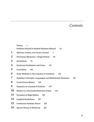
37. NEWTONIAN MECHANICS—SINGLE PARTICLE 33
1 2
y = y0 − gt (2)
2
where y0 = 80 m , and we need to solve for x0 . From (2), the time the bale hits the ground is
τ = 2 y0 g . If we want the bale to land at x (τ ) = −30 m , then x0 = x (τ ) − v0τ . Substituting
v0 = 44.4 m ⋅ s -1 and the other values, this gives x0 −210 m . The rancher should drop the bales
210 m behind the cattle.
b) She could drop the bale earlier by any amount of time and not hit the cattle. If she were late
by the amount of time it takes the bale (or the plane) to travel by 30 m in the x-direction, then
she will strike cattle. This time is given by ( 30 m ) v0 0.68 s .
2-7. Air resistance is always anti-parallel to the velocity. The vector expression is:
1  v 1
W= cw ρ Av 2  −  = − cw ρ Avv (1)
2  v 2
Including gravity and setting Fnet = ma , we obtain the parametric equations
x = − bx x 2 + y 2 (2)
y = −by x 2 + y 2 − g (3)
where b = cw ρ A 2m . Solving with a computer using the given values and ρ = 1.3 kg ⋅ m -3 , we
find that if the rancher drops the bale 210 m behind the cattle (the answer from the previous
problem), then it takes 4.44 s to land 62.5 m behind the cattle. This means that the bale
should be dropped at 178 m behind the cattle to land 30 m behind. This solution is what is
plotted in the figure. The time error she is allowed to make is the same as in the previous
problem since it only depends on how fast the plane is moving.
80
60
y (m)
40
20
0
–200 –180 –160 –140 –120 –100 –80 –60 –40
x (m)
With air resistance
No air resistance