Asset Impairment Test Sensitivity Analysis

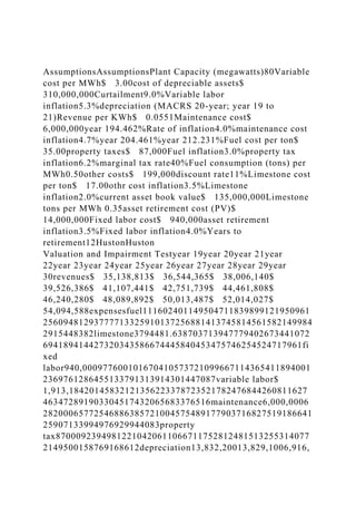
AssumptionsAssumptionsPlant Capacity (megawatts)80Variable
cost per MWh$ 3.00cost of depreciable assets$
310,000,000Curtailment9.0%Variable labor
inflation5.3%depreciation (MACRS 20-year; year 19 to
21)Revenue per KWh$ 0.0551Maintenance cost$
6,000,000year 194.462%Rate of inflation4.0%maintenance cost
inflation4.7%year 204.461%year 212.231%Fuel cost per ton$
35.00property taxes$ 87,000Fuel inflation3.0%property tax
inflation6.2%marginal tax rate40%Fuel consumption (tons) per
MWh0.50other costs$ 199,000discount rate11%Limestone cost
per ton$ 17.00othr cost inflation3.5%Limestone
inflation2.0%current asset book value$ 135,000,000Limestone
tons per MWh 0.35asset retirement cost (PV)$
14,000,000Fixed labor cost$ 940,000asset retirement
inflation3.5%Fixed labor inflation4.0%Years to
retirement12HustonHuston
Valuation and Impairment Testyear 19year 20year 21year
22year 23year 24year 25year 26year 27year 28year 29year
30revenues$ 35,138,813$ 36,544,365$ 38,006,140$
39,526,386$ 41,107,441$ 42,751,739$ 44,461,808$
46,240,280$ 48,089,892$ 50,013,487$ 52,014,027$
54,094,588expensesfuel111602401149504711839899121950961
25609481293777713325910137256881413745814561582149984
2915448382limestone3794481.638703713947779402673441072
694189414427320343586674445840453475746254524717961fi
xed
labor940,000977600101670410573721099667114365411894001
2369761286455133791313914301447087variable labor$
1,913,18420145832121356223378723521782476844260811627
463472891903304517432065683376516maintenance6,000,0006
28200065772546886385721004575489177903716827519186641
25907133994976929944083property
tax87000923949812210420611066711752812481513255314077
2149500158769168612depreciation13,832,20013,829,1006,916,

100000000000other199000205,965.0213,173.8220,634.9228,35
7.1236,349.6244,621.8253,183.6262,045.0271,216.6280,709.22
90,534.0total
expenses37926105.6387670603273038726724215276691322865
0483296697823072860431828598329714803415904835393175i
ncome before taxes$ (2,787,293)$ (2,222,695)$ 5,275,753$
12,802,170$ 13,438,309$ 14,101,255$ 14,792,026$
15,511,676$ 16,261,294$ 17,042,007$ 17,854,979$
18,701,413taxes$ (1,114,917)$ (889,078)$ 2,110,301$
5,120,868$ 5,375,324$ 5,640,502$ 5,916,810$ 6,204,670$
6,504,518$ 6,816,803$ 7,141,991$ 7,480,565net income$
(1,672,376)$ (1,333,617)$ 3,165,452$ 7,681,302$
8,062,986$ 8,460,753$ 8,875,216$ 9,307,006$ 9,756,776$
10,225,204$ 10,712,987$ 11,220,848add
depreciation13,832,20013,829,1006,916,100- 0- 0- 0- 0- 0- 0- 0-
0- 0less asset retirement cost- 0- 0- 0- 0- 0- 0- 0- 0- 0- 0-
0($12,692,977)after tax net cash flow$ 12,159,824$
12,495,483$ 10,081,552$ 7,681,302$ 8,062,986$
8,460,753$ 8,875,216$ 9,307,006$ 9,756,776$
10,225,204$ 10,712,987$ (1,472,129)totol future cash flows$
106,346,960Present value of cashflows$ 61,543,280current
book value$ 135,000,000impairedYES!!!Write down required$
73,456,720
Training Plan Template
Student Name:
_________________________________________
Date: ________________________________________________
Training Plan Template
Introduction
(Describe the purpose of the training program)
Scope

(Describe the scope of the training, such as initial training for
new employees, staff training on important topics, etc.)
Objectives
(Describe the objectives or expected results of the training.
Express objectives as actions that the users will be expected to
perform once they have been trained.)
Background
(Provide an overview of the training curriculum.)
Training Requirements
(The training audience and the time frame in which training
must be accomplished.)
Training Strategy
(What steps will you take in planning the program?)
Training Evaluation
(Describe how training evaluation will be performed using the
Kirkpatrick levels)
Training Methods
(What training methods will you use and why)
Training Delivery
Constraints/Limitations
(Identify all known constraints and/or limitations that could
potentially affect the training.)

(Given the situation, what would be the best way to deliver the
training? Why?)
Use the model to assess the sensitivity of the impairment test re
sults by simply changing the assumptions entered on the
“Assumptions” worksheet and observing
the changes in the projected cash flows and the indicated
impairment write-down amount, if any. Before you complete
Scenario #1, make sure all of your Assumptions match their
original values as seen in Exhibit #1.
Scenario #1
Assumption Name:
Revised Assumption:
Curtailment
9%
Revenue per KWh
.0551
Variable labor inflation
5.3%
Limestone consumption (tons) per MWh
0.35
What are the total future cash flows based on the revised
assumptions in Scenario #1?
$118553589
2 points
QUESTION 2

Based on the assumptions in Scenario #1, the asset is impaired.
True, the asset is impaired since the present value of cash flows
amounts to 61281111 while the current book value is
135000000
1 points
QUESTION 3
sults by simply changing the assumptions entered on
the “Assumptions” worksheet and observing
Scenario #1
Assumption Name:
Revised Assumption:
Curtailment
9%
Revenue per KWh
.0551
5.3%
0.35
If the asset is impaired, what is the required write down based
on the revised assumptions in Scenario #1 (answer as a positive
number)? If a write down is not required, answer 0.
. $ 73718889
2 points

QUESTION 4
Scenario #2
Assumption Name:
Revised Assumption:
Limestone cost per ton
17
Fixed labor cost
940,000
Maintenance inflation
4.7%
Asset retirement inflation
3.5%
. $ 120219582
2 points
QUESTION 5
True, the asset is impaired since the present value of cash flows
(61951284), is lower than the current book value of 135000000
1 points
QUESTION 6

Scenario #2
Assumption Name:
Revised Assumption:
17
Fixed labor cost
940,000
4.7%
3.5%
. Required write down $ 73048716
2 points
QUESTION 7
Scenario #3

Assumption Name:
Revised Assumption:
Fuel cost per ton
35
Property tax inflation
6.2%
Other costs
199,000
Discount rate
11%
. $ 106346960
2 points
QUESTION 8
True, it is impaired since its present value of cash flows is $
61543280 and the current book value is 135000000
1 points
QUESTION 9
Scenario #3
Assumption Name:
Revised Assumption:

Fuel cost per ton
35
6.2%
Other costs
199,000
Discount rate
11%
. $ 73456720
2 points
Click Save and Submit to save and submit. Click Save All
Answers to save all answers.
ACC340 External Financial Reporting
Case 4: Excel Assignment – Asset Impairment
Fall, 2016
1
Excel is a powerful tool for financial modeling and analysis.
Accordingly, it is vital for financial and
accounting professionals to develop their skills with the
software to enhance their efficiency and
effectiveness. The objective of this assignment is to provide
hands-on experience creating a financial
model that will be used to perform an impairment test on an

asset.
For the purpose of this assignment, you are to assume that you
work for Pacific Energy Company and
have been tasked with performing impairment tests on a number
of the company’s assets. One such
asset is an 80 megawatt cogeneration power plant that is fueled
by biomass. This particular plant
generates high pressure steam used to generate electricity by
burning the waste byproduct resulting
from timber processing and paper manufacturing. Once high-
pressure steam is used to generate
electricity, the residual low-pressure steam is used by an
adjacent paper mill to produce paper and heat
its plant (the dual use of high and low pressure steam is referred
to as cogeneration). Because of this
relationship with the paper mill, the energy plant is able to
purchase biomass fuel at lower than market
rates.
Due to declining energy rates and higher than expected
curtailment (will be explained later), the plant’s
revenue has diminished and competitive forces in the energy
market are expected to continue this
trend. Accordingly, Pacific Energy is concerned that the plant
asset may be impaired. You have been
tasked with creating a discounted cash flow model that can be
used to determine if the asset is impaired
and the sensitivity of the assumptions made too perform the
test.
The plant was permitted by the Federal Energy Regulatory
Commission (FERC) to operate for 30 years.
You are preparing the impairment test at the end of its
eighteenth year of operation. The plant had an
original cost of $320 million, $10 million of which was

attributed to the land the plant is sited on.
Depreciable assets ($310 million) are being depreciated for
financial reporting purposes on a straight-
line basis over the plant’s permitted life of 30 years with no
residual value, and over 20 years for tax
purposes. An asset retirement obligation was capitalized and has
a current estimated value of $14
million. The plant’s assets are evaluated together (including
land) for the purposes of impairment testing
and have a combined book value $135 million. Additional
information about the plant will be provided in
the instructions that follow.
To get started with the impairment analysis, open a new Excel
workbook and save it with the following
name (“YOUR LAST NAME - Pacific Energy Asset Impairment
Test ”). My project file name would be
“HUSTON - Pacific Energy Asset Impairment Test”. Make sure
that you save your file frequently as you
work through this assignment.
When you build a spreadsheet model, it is best to have one area
in which you input the assumption
variables used to derive the amounts in the rest of the model.
This allows you to easily change your
assumptions and evaluate the effect those changes had on your
results. This is known as “sensitivity
analysis”.
Fall, 2016

2
You will notice that there are tabs at the bottom left of the
screen that are currently labeled as “Sheet
1”, “Sheet 2”, and “Sheet 3”. Additional sheets can be added to
the workbook, however, you will only be
using two sheets for our project. Accordingly, we will delete the
sheet that we do not need. To do so,
right click on the tab labeled “Sheet 3” and select “Delete” from
the menu that appears. Now you will
rename the other two tabs by right clicking on them and
selecting the “Rename” on the menu that
appears, typing the desired name and pressing enter. Rename
“Sheet 1” as “Assumptions” and “Sheet
2” as “Valuation & Impairment Test”.
Please note that if you make a mistake while performing an
operation in Excel, you can reverse the
action by clicking on the button in the upper left part of the
screen that features a circular shaped blue
arrow. This is the “Back” or “Undo” button and can be used to
walk back through several of the most
recently performed operations.
Now you will construct the assumptions worksheet, so click on
the “Assumptions” tab to make sure you
are on the correct sheet. At the top of the sheet, in cell A1, type
in the word “Assumptions” and press
enter (notice that you can click on the check mark in the
navigation bar just above the alpha character
column headings; doing so is the same as pressing enter after
inputting or editing data in a cell). In cell

A3, type the label “Plant capacity (megawatts)” and press enter
(or click on the check mark). To adjust
the column so that it is wide enough to display the label, move
your mouse pointer so that is over the
line on the right side of the column A heading. Your pointer
should change in appearance from an
arrowhead to a vertical line with arrows pointing right and left.
While the pointer is in this mode,
double-click the left mouse button and the column width will
automatically adjust to the needed width
to display the widest entry in the column. Now, in cell B3, enter
the number 80. To make sure that
numbers are formatted in a consistent manner, locate the button
with a comma on it in the tool bar (it
should be in the tool bar section labeled “Number”). Click on
the button and confirm that the amount
entered in the cell is displayed with two decimal places, which
is the default number of decimal places
for the comma format. An alternative to accessing formatting
tools via the toolbar is to right click on the
cell to be formatted and selecting the desired action from the
tool bar / menu that appears.
In cell A4, enter the label “Curtailment”. Like most
cogeneration plants, this plant is an independent
power producer meaning that it is not part of a major utility.
Instead, it produces energy and sells it to
the local utility. When demand for electricity is lower and
within the capacity of the local utility, Pacific’s
plant is told to stop generating electricity. This is referred to as
curtailment (curtail energy production).
At the time that Pacific built the plant, curtailment was assumed
to be 4%. Given current curtailment
rates and the expected trend for the future, Pacific now
estimates curtailment will be 10% for the
remainder of the plant’s life. In cell B4, enter .10 and click on

the check mark button or press enter.
Next, locate the “%” button on the tool bar (next to the comma
button). Click on the button and confirm
that the amount entered is now displayed as “10%”. There are
times when the curtailment assumption
will be indicated in tenths of a percent. To prepare for this
possibility, while your cell pointer is on cell
B4, click the button on the tool bar that shows .0 above .00 with
an arrow pointing to the left one time.
Each time you click on this button, the number of decimal
places displayed for the highlighted cell (or
Fall, 2016
3
cells) increase by one decimal place. After clicking one time on
the button with cell B4 highlighted, its
contents should be displayed as “10.0%”. If you accidentally
increased the number of decimal places to
more than one, you can decrease the number of decimal places
displayed by clicking on the button that
shows “.00” above “.0” with an arrow pointing to the right.
Each time this button is clicked, the number
of decimals displayed is decreased by one. Please note that if
any of the cells in your worksheet displays
a series of pound signs (########), Excel is indicating that an
entered number or formula result is too

wide to be displayed with the current column width setting. If
this happens, simply adjust the column
width as previously discussed.
In cell A6, enter the label “Revenue per KWh” and press enter.
In cell B6, enter the amount .0549 and
press enter. Locate the button on the tool bar that is labeled
with the dollar sign ($) to change the
format to currency. While highlighting cell B6, click on this
button and increase the number of decimal
places displayed to four. The contents of cell B6 should now be
displayed as “$0.0549”. In cell A7, enter
the label “Rate inflation” and press enter. In cell B7, enter the
amount .04. Format the cell to display
percent with one decimal place.
In cell A9, enter the label “Fuel cost per ton” and press enter. In
cell B9, enter the amount “30”. Format
the cell to display currency with two decimal places. In cell
A10, enter the label “Fuel inflation” and
press enter. In cell B10, enter the amount .03. Format the cell to
display percent with one decimal place.
In cell A11, enter the label “Fuel consumption (tons) per MWh”
and press enter. Notice that the
contents of cell A11 are larger than what the previously
adjusted column width can accommodate. To
adjust the column, we will use a different approach. Go again to
the top of the column and place your
mouse pointer over the right line in column A heading. Once
your mouse pointer changes to the vertical
line with opposing arrows, click and drag the mouse to the right
to increase the column width to 31.44
points (a display will pop up and indicate the column width
setting). In cell B11, enter the amount .5. Set
the cell to the comma display format with two decimal places.

Limestone is used in the burning of biomass to enhance
combustion and reduce emissions. In cell A13,
enter the label “Limestone cost per ton”. In cell B13, enter the
amount 18 and press enter. Format the
cell to display currency with two decimal places. In cell A14,
enter the label “Limestone inflation”. In cell
B14, enter the amount .02 and format the cell to display percent
with one decimal place. In cell A15,
enter, the label “Limestone consumed (tons) per MWh”. In cell
B15, enter the amount .15 and format
the cell using the comma button with two decimal places
displayed.
In cell A17, enter the label “Fixed labor cost”. In cell B17,
enter the amount 1000000 ($1 million) and
format the cell to display currency with zero decimal places.
Automatically set the width of column B by
double-clicking on the right side vertical line in the column B
heading. In cell A18, enter the label “Fixed
labor inflation”. In cell B18, enter the amount .04 and format
the cell to display percent with one
decimal place.
Fall, 2016
4
In cell D3, enter the label “Variable cost per MWh”.

Automatically set the width of column D by double-
clicking on the right side vertical line in the column D heading.
In cell E3, enter the amount 3 and format
the cell as currency with two decimal places. In cell D4, enter
the label “Variable labor inflation”. In cell
E4 enter the amount .045 and format the cell to display percent
with one decimal place.
In D6, enter the label “Maintenance cost”. In cell E6, enter the
amount 6000000 ($6 million) and format
the cell to display currency with zero decimal places. In cell
D7, enter the label “Maintenance cost
inflation”. In cell E7, enter the amount .04 and format the cell
to display percent with one decimal place.
In D9, enter the label “Property taxes”. In cell E9, enter the
amount 87000 and format the cell to display
currency with zero decimal places. In cell D10, enter the label
“Property tax inflation”. In cell E10, enter
the amount .05 and format the cell to display percent with one
decimal place.
In D12, enter the label “Other costs”. In cell E12, enter the
amount 172000 and format the cell to display
currency with zero decimal places. In cell D13, enter the label
“Other costs inflation”. In cell E13, enter
the amount .035 and format the cell to display percent with one
decimal place. Before moving on, enter
your first name in cell JK103.
Assets such as power plants require significant costs to be
incurred to take them out of service. These
expenditures are known as “asset retirement costs” and must be
included in the cash flow projections
used for the purpose of impairment testing. In cell D16, enter
the label “Asset retirement cost (PV)”. The

label indicates that the amount that will be entered is the
present, or current, value of the retirement
costs, not the expected cost to be incurred in twelve years when
the plant is taken out of service. The
amount will be adjusted to reflect the anticipated future cost.
Manually adjust the width of column D to
31.44 points by clicking on the right side vertical line in the
column heading and dragging it to the right.
In cell E16, enter the amount 14000000 ($14 million) and
format the cell to display currency with zero
decimal places. In cell D 17 enter the label “Asset retirement
inflation”. In cell E17, enter the amount
.045 and format the cell to display percent with one decimal
place. In cell D18, enter the label “Years to
retirement”. In cell E18, enter the amount 12 and format the cell
with commas and no decimal places.
In cell G3, enter the label “Cost of depreciable assets” and
manually adjust the width of column G to
31.44 points. As discussed above, the historical cost of the plant
is $320 million, which includes the $10
million cost of the land the plant is sited on. Therefore, the cost
of depreciable assets is $310 million.
Enter this amount, 310000000, in cell H3 and format the cell for
currency with no decimal places
displayed. Automatically adjust the width of column H to fit the
amount entered for depreciable cost.
Power plant assets are 20-year class assets for tax depreciation
purposes (which is the depreciation we
must calculate for the effect it has on after tax cash flows). IRS
MACRS tax depreciation assumes a mid-
year convention, meaning that it allows one half year of
depreciation in the year an asset is placed in
service and one half year of depreciation in the last year of
depreciation is taken (year 21). As stated

previously, the power plant has been in service for 18 years
(and is permitted by the FERC to operate for
30 years). Therefore, for tax purposes there are three years of
depreciation remaining (year 19, year 20,
Fall, 2016
5
and a half year in year 21). In cell G5, enter the label
“Depreciation (MACRS 20-Year; years 19 to 21)”. In
cell G6, enter the label “Year 19”, in cell G7, enter the label
“Year 20”, and in cell G8 enter the label
“Year 21”. In cell H6, enter the amount .04462, in cell H7 enter
the amount .04461, and in cell H8 enter
the amount .02231. Highlight the cells H6, H7, and H8 and
format the cells to display percent with three
decimal places.
In cell G10, enter the label “Marginal tax rate”. In cell H10,
enter the amount .4 and format the cell to
display percent with no decimal places.
In cell G12, enter the label “Discount rate”. In cell H12, enter
the amount .135 and format the cell to
display percent with one decimal place.
In cell G14, enter the label “Current asset book value”. In cell

H14, enter the amount 135000000 ($135
million) and format the cell to display currency with zero
decimal places.
To finalize the assumptions sheet, click on cell A1 and highlight
to cell H1. Locate and click on the
“Merge & Center” button on the tool bar (located in the
“Alignment” section). This will merge cells A1 to
H1 into one large cell and center the label that was entered in
cell A1 in the new merged cell. Now click
on boldfaced “B” button in the “Font” section of the tool bar.
Lastly, click on the down-pointing arrow
next to the font size number to display the available font size
options and click on “14” to change the
font size to 14 points. You are now finished with creating and
formatting the assumptions portion of the
impairment model. Take a few moments to compare your
worksheet to the one pictured in Exhibit #1 at
the end of this document to make sure it looks correct. Before
moving on, enter your last name in cell
KT342.
Now you will construct the cash flow projection for the
remaining life of the plant. Click on the tab for
the “Valuation & Impairment Test” worksheet. Manually set the
width of column A to 25.33 points.
Next you will set the width of columns B through M to 13.00
points. To do so, place your mouse pointer
over the area of the column B heading. Notice that the mouse
pointer changes to a thick down pointing
arrow. Click and hold the left mouse button down and drag your
mouse from the heading for column B
to the heading for column M and release the left mouse button.
Columns B through M should now be
highlighted. Locate and click on the “Format” button on the tool
bar (in the “Cells” section of the tool

bar). Select the “Column width” option from the drop down
menu, enter 13 in the input field, and click
the “OK” button.
In cell B2, enter the label “Year 19” and boldface the font. Also
click on the button on the tool bar that
has a “U” with a line below it to underline the label. With cell
B2 selected, notice that the outline of the
cell has a small black square on the bottom right corner. This is
referred to as a “handle”. Click on the
handle and drag it to the right until you have highlighted
through cell M2 (notice as you do so, Excel
indicates the year number that it will automatically fill to as
you go). This should copy the label in cell
B2 to cells C2 through M2, adjusting along the way so that your
spreadsheet now displays column
labels for years 19 through 30.
Fall, 2016
6
In cell A4, enter the label “Revenues”. In cell B4 you will enter
a formula that references the
assumptions entered in the” Assumptions” sheet to calculate the
expected revenue for year 19. The
formula will multiply the plant’s capacity times a factor that
adjusts for curtailment (the time the plant is

not generating power) times the energy rate (Revenue per
KWh), times 1,000 (to convert KWhs to
megawatts), times 24 hours per day, times 365 days per year. To
start the process, click on the cell (B4 in
the “Valuation & Impairment Test” worksheet) and enter an
equal sign (=) (do not press the enter key at
this time). Next click on the “Assumptions” sheet tab and click
on the Plant Capacity cell (B3). Next,
enter an asterisk (*) to indicate multiplication. Enter a right
facing parenthesis “(“ and the number one
(1). Enter a minus sign (-) and click on the curtailment
percentage in cell B4. Now enter a left facing
parenthesis “)” and an asterisk to indicate multiplication. Click
on the Revenue per KWh cell in B6 and
enter an asterisk for multiplication. Enter 1000 and enter an
asterisk. Enter 24 and enter an asterisk.
Enter 365 and press the enter key. Click on cell B4 in the
“Valuation & Impairment Test” worksheet and
format the cell to display currency with zero decimal places.
Your worksheet should display year 19
revenues of $34,626,528. If this is not the case, click on cell B4
and review your formula displayed in the
cell contents field just below the tool bar. It should be:
=Assumptions!B3*(1-
Assumptions!B4)*Assumptions!B6*1000*24*365
If it is not, edit the formula as needed in the cell contents field
and press enter.
Next you will enter a formula in cell C4 that will estimate
revenues for year 20 by increasing the
estimated revenues for year 19 by the amount by which energy
rates are expected to inflate each year.
To do so, click on the cell (C4 in the “Valuation & Impairment

Test” worksheet) and enter an equal sign
(=). Click on the year 19 revenue cell (B4 in the “Valuation &
Impairment Test” worksheet). Enter an
asterisk to indicate multiplication. Enter a right facing
parenthesis “(“ and the number one (1). Enter the
plus sign (+) and click on the tab to navigate to the
“Assumptions” worksheet. Click on the rate inflation
factor in cell B7. Enter a left facing parenthesis “)”, press enter,
and format cell C4 to display currency
with zero decimal places. Your spreadsheet should display year
20 revenues of $36,011,589. As
discussed above, review your formula and make needed
adjustments so that it is stated as:
=B4*(1+Assumptions!B7)
Before copying the formula to cells D4 through M4, we must
make an adjustment so that it copies
correctly. Once a formula is created, it can be copied to other
cells where it will perform the same
operation. If a formula is entered that tells Excel to add the
number in the cell one row above and one
column to the left to the amount in the cell one row below and
one column to the right, it will perform
that operation wherever it is copied to. This is called relative
cell referencing, which is where Excel
automatically adjusts the cell references (column letter and row
number) so that formula elements are
referencing the correct cells wherever the formula is copied to.
This is fine in many cases, however,
there are times when it is not. In the formula above, you
instructed Excel to multiply the amount in the
cell one position to the left of cell B5 by the amount in the rate
inflation factor cell in the “Assumptions”

Fall, 2016
7
worksheet. If this formula is copied to cell D4, it will multiply
the amount one cell to the left in cell C4,
which is correct, by the amount in the cell next to the one in
which the rate inflation factor is stored in
the “Assumptions” worksheet. The problem is that we need the
formula to always reference the cell
containing the rate inflation factor on the “Assumptions” page,
no matter where the formula is copied
to. This is referred to as “absolute cell referencing”, which is
where we tell Excel to not automatically
adjust the cell references for a formula element when it is
copied to other cells. To modify the formula,
click on cell C4. In the cell contents display field, click on the
portion of the formula that states “B7”.
Now press the F4 key on your keyboard. Notice that each time
you press the F4 key, Excel places
different combinations of dollar signs ($) in front of the column
letter and row number. The dollar sign is
used by Excel to indicate that a particular portion of a formula
is not to be altered when it is copied. We
will be copying the formula laterally across the row 4 of the
worksheet. This would cause Excel to
automatically adjust the column letter in the formula, which we

do not want to happen. Accordingly, a
dollar sign must be in front of the column indicator. Press the
F4 key until this is the case and then press
enter when done. Your formula should be stated as:
=B4*(1+Assumptions!$B7)
Now you are ready to copy the formula to cells D4 through M4.
To do so, click on the “handle” on the
lower right corner of the cell pointer (with the pointer on cell
C4) and drag the cell indicator to cell M4
and release. Your formula should be copied to the cells in the
range and your worksheet should be
displaying year 30 revenues of $53,305,949. If this is not the
case, review the formula that you copied in
cell C4, make necessary adjustments and copy the formula again
to cells D4 through M4.
Next you will enter estimates for expenses for years 19 through
30. Click on cell A6 and enter the label
“Expenses:”. Click on cell A7 and enter the label “Fuel”.
In cell B7 you will enter a formula that calculates the cost of
the fuel the plant will consume in one year.
To do so, the formula will multiply the plant capacity times one
minus the curtailment rate (to adjust for
the amount of time it is expected the plant will be off-line and
not generating electricity or consuming
fuel), times the cost of fuel per ton, times the fuel consumption
rate per megawatt hour, times 24 hours,
times 365 days. To get started, click on cell B7 and enter an
equal sign. Navigate to the “Assumptions”
worksheet and click on the plant capacity in cell B3. Enter an
asterisk and a right facing parenthesis.

Enter the number one and a minus sign. Click on the curtailment
factor in cell B4 and enter a left facing
parenthesis. Enter an asterisk and click on the fuel cost per ton
in cell B9. Enter an asterisk and click on
the fuel consumption rate in cell B11 and then enter another
asterisk. Enter the number 24, another
asterisk, and then the number of 365. Press the enter key and
format the cell to display currency with
zero decimal places. Your worksheet should display $9,460,800
as the fuel cost for year 19. If this is not
the case, make appropriate edits to the formula so that it is
stated as:
=Assumptions!B3*(1-
Assumptions!B4)*Assumptions!B9*Assumptions!B11*24*365
Fall, 2016
8
In cell C7, you will enter a formula that increases the annual
cost of fuel consumed in year 19 by the
assumed fuel inflation rate. To do so, click on cell C7 and enter
an equal sign. Click on cell B7 and then
enter an asterisk. Enter a right facing parenthesis and the
number one. Enter a plus sign and then
navigate to the “Assumptions” worksheet. Click on the fuel

inflation factor in cell B10 and indicate
absolute cell referencing for the cell’s column indicator (place a
dollar sign in front of the “B” in the cell
address “B10”). Enter a left facing parenthesis and press the
enter key. Format cell C7 so that it is
displaying currency with no decimal places. Your spreadsheet
should state year 20 fuel expense of
$9,744,624. If this is not the case, make appropriate edits to the
formula so that it is stated as:
Copy the formula in cell C7 to cells D7 though M7. Your
spreadsheet should indicate year 30 fuel
expense of $13,095,960. If this is not the case, review the
formula in cell C7, make necessary edits and
copy the revised formula to the desired cells.
In cell A8, enter the label “Limestone”. In cell B8, you will
enter a formula that calculates the annual cost
of limestone consumed by the plant. To do so, the formula will
multiply the plant capacity times one
minus the curtailment rate, times the cost of limestone per ton,
times the limestone consumption rate
per megawatt hour, times 24 hours, times 365 days. To get
started, click on cell B8 and enter an equal
sign. Navigate to the “Assumptions” worksheet and click on the
plant capacity in cell B3. Enter an
asterisks and a right facing parenthesis. Enter the number one
and a minus sign. Click on the curtailment
factor in cell B4 and enter a left facing parenthesis. Enter an
asterisk and click on the limestone cost per
ton in cell B13. Enter an asterisk and click on the limestone
consumption rate in cell B15 and then enter

another asterisk. Enter the number 24, another asterisk, and then
the number of 365. Press the enter
key and format the cell to display commas with zero decimal
places. Your worksheet should display
$1,702,944 as the limestone cost for year 19. If this is not the
case, make appropriate edits to the
=Assumptions!B3*(1-
Assumptions!B4)*Assumptions!B13*Assumptions!B15*24*365
cost of limestone consumed in year 19 by
the assumed limestone inflation rate. To do so, click on cell C8
and enter an equal sign. Click on cell B8
and then enter an asterisk. Enter a right facing parenthesis and
the number one. Enter a plus sign and
then navigate to the “Assumptions” worksheet. Click on the
limestone inflation factor in cell B14 and
indicate absolute cell referencing for the cell’s column indicator
(place a dollar sign in front of the “B” in
the cell address “B14”). Enter a left facing parenthesis and
press the enter key. Format cell C8 so that it
is displaying commas with no decimal places. Your spreadsheet
should state year 20 limestone expense
of $1,737,003. If this is not the case, make appropriate edits to
the formula so that it is stated as:

Fall, 2016
9
spreadsheet should indicate year 30 limestone
In cell A9, enter the label “Fixed labor”. In cell B9, enter an
equal sign and then navigate to the
“Assumptions” worksheet. Select the fixed labor cost in cell
B17 and press enter. Format the cell to
display commas with zero decimal places. Next you will enter a
formula in cell C9 that increases year 19
estimated fixed labor cost by the assumed fixed labor inflation
factor. To do so, select cell C9 and enter
an equal sign. Click on cell B9 and enter an asterisk. Enter a
right facing parenthesis and the number
one. Enter a plus sign and then navigate to the “Assumptions”
worksheet and select the fixed labor
inflation factor in cell B18. Indicate absolute cell referencing
for the column indicator and then enter a
left facing parenthesis. Your spreadsheet should state year 20
fixed labor expense of $1,040,000. If this
is not the case, make appropriate edits to the formula so that it
is stated as:

spreadsheet should indicate year 30 fixed labor
In cell A10, enter the label “Variable labor”. In cell B10, you
will enter a formula that calculates the
annual cost of variable labor needed to operate the plant. To do
so, the formula will multiply the plant
capacity times one minus the curtailment rate, times the cost of
variable labor per megawatt hour,
times 24 hours, times 365 days. To get started, click on cell B10
and enter an equal sign. Navigate to the
“Assumptions” worksheet and click on the plant capacity in cell
B3. Enter an asterisk and a right facing
parenthesis. Enter the number one and a minus sign. Click on
the curtailment factor in cell B4 and enter
a left facing parenthesis. Enter an asterisk and click on the cost
of variable labor per MWh in cell E3.
Enter the number 24, another asterisk, and then the number of
365. Press the enter key and format the
cell to display commas with zero decimal places. Your
worksheet should display $1,892,160 as the
variable labor cost for year 19. If this is not the case, make
appropriate edits to the formula so that it is
stated as:
=Assumptions!B3*(1-
Assumptions!B4)*Assumptions!E3*24*365
cost of variable labor estimated for year 19

by the assumed variable labor cost inflation rate. To do so, click
on cell C10 and enter an equal sign.
Click on cell B10 and then enter an asterisk. Enter a right facing
parenthesis and the number one. Enter a
plus sign and then navigate to the “Assumptions” worksheet.
Click on the variable labor inflation factor
in cell E4 and indicate absolute cell referencing for the cell’s
column indicator (place a dollar sign in front
of the “E” in the cell address “E4”). Enter a left facing
parenthesis and press the enter key. Format cell
C10 so that it is displaying commas with no decimal places.
Your spreadsheet should state year 20
Fall, 2016
10
variable labor expense of $1,977,307. If this is not the case,
make appropriate edits to the formula so
that it is stated as:
=B10*(1+Assumptions!$E4)
spreadsheet should indicate year 30 variable
labor expense of $3,070,698. If this is not the case, review the
formula in cell C10, make necessary edits

and copy the revised formula to the desired cells.
In cell A11, enter the label “Maintenance”. In cell B11, enter an
“Assumptions” worksheet. Select the maintenance cost in cell
E6 and press enter. Format the cell to
estimated maintenance cost by the assumed maintenance cost
inflation factor. To do so, select cell C11
and enter an equal sign. Click on cell B11 and enter an asterisk.
Enter a right facing parenthesis and the
number one. Enter a plus sign and then navigate to the
“Assumptions” worksheet and select the
maintenance cost inflation factor in cell E7. Indicate absolute
cell referencing for the column indicator,
enter a left facing parenthesis and press enter. Your spreadsheet
should state year 20 maintenance
expense of $6,240,000. If this is not the case, make appropriate
edits to the formula so that it is stated
as:
spreadsheet should indicate year 30
maintenance expense of $9,236,724. If this is not the case,
review the formula in cell C11, make
necessary edits and copy the revised formula to the desired
cells.
In cell A12, enter the label “Property tax”. In cell B12, enter an
“Assumptions” worksheet. Select the property tax cost in cell

E9 and press enter. Format the cell to
estimated property tax expense by the assumed property tax
inflation factor. To do so, select cell C12
and enter an equal sign. Click on cell B12 and enter an asterisk.
Enter a right facing parenthesis and the
number one. Enter a plus sign and then navigate to the
“Assumptions” worksheet and select the
property tax inflation factor in cell E10. Indicate absolute cell
referencing for the column indicator and
then enter a left facing parenthesis. Your spreadsheet should
state year 20 property tax expense of
$91,350. If this is not the case, make appropriate edits to the
spreadsheet should indicate year 30
property tax expense of $148,800. If this is not the case, review
the formula in cell C12, make necessary
edits and copy the revised formula to the desired cells.
Fall, 2016
11

In cell A13, enter the label “Depreciation”. In cell B13, enter an
“Assumptions” worksheet. Select the cost of depreciable assets
in cell H3. Enter an asterisk and then
select the year 19 depreciation factor in cell H6. Press enter and
format the cell to display commas with
zero decimal places. In cell C13, enter a formula that multiplies
the cost of depreciable assets (on the
“Assumptions” worksheet) by the depreciation factor for year
20. Format the cell to display commas
with no decimal places. Do the same for year 21. For year 22,
enter a zero and format the cell to display
commas (note that for this format option, Excel displays a dash
(-) for values of zero. Copy cell E13 to
cells F13 though M13. Your worksheet should indicate
depreciation expense of $13,832,200,
$13,829,100, and $6,916,100 for year 19, year 20, and year 21
respectively. If that is not the case, revisit
your formulas for the related cells and make necessary
adjustments. The formula for cell B13 should be
as follows:
=Assumptions!H3*Assumptions!H6
In cell A14, enter the label “Other”. In cell B14, enter an equal
sign and then navigate to the
“Assumptions” worksheet. Select the assumption for other costs
in cell E12 and press enter. Format the
cell to display commas with zero decimal places. Next you will
enter a formula in cell C14 that increases
year 19 estimated other expense by the other costs inflation
factor. To do so, select cell C14 and enter
an equal sign. Click on cell B14 and enter an asterisk. Enter a

right facing parenthesis and the number
one. Enter a plus sign and then navigate to the “Assumptions”
worksheet and select the other costs
inflation factor in cell E13. Indicate absolute cell referencing
for the column indicator and then enter a
left facing parenthesis. Your spreadsheet should state year 20
other expense of $178,020. If this is not
the case, make appropriate edits to the formula so that it is
stated as:
spreadsheet should indicate year 30 other
expense of $251,115. If this is not the case, review the formula
in cell C14, make necessary edits and
The expense section of the forecast is now complete (income
taxes are presented lower in the
projection). For formatting purposes, a line should be placed
below this section at the bottom of cells
B14 through M14. To do this, select this range of cells by
clicking on cell B14 and dragging your mouse to
the right while depressing the left mouse button. Release the
button once you have highlighted the
desired range of cells. Locate the button on the toolbar that
looks like a box with a line at the bottom of
it (located in the “Font” section of the toolbar). Click on the
button and Excel will place a line at the
bottom of the cells in the range you selected. You may have to
click on a cell outside of the range to see
the line. To remove the line or select a different type of line,
you would highlight the range and click on

the down pointing arrow next to the toolbar button used a
moment ago to add the line, and then select
the desired format. Take a moment to explore the line options
available with this formatting tool.
Fall, 2016
12
In cell A16, enter the label “Total expenses”. Select cell B16
and click on the “AutoSum” button on the
toolbar (located in the “Editing” section of the toolbar). Make
sure that the “AutoSum” wizard highlights
cells B7 though B15. If this is not the case, use the blue
“handles” on the corners of the range indicator
box to adjust the box dimensions to highlight the correct cells.
Once you confirm the correct cells are
being summed, press enter. Select cell B16 and notice the
function that was created in the cell contents
display area (just below the toolbar). The AutoSum wizard
entered the function “ =SUM(B7:B15)” for
you. If you wanted to, you could have entered an equal sign, the
word “SUM” and a right facing
parenthesis in the cell, and then highlighted the desired range of
cells and entered a left facing
parenthesis to create the function. Obviously, the AutoSum
wizard is a time saver that speeds up the
entry of a very commonly used function. Now, format cell B16

to display currency with no decimal
places and copy it to cell C16 though cell M16. Your
spreadsheet should indicate total expenses for year
19 and year 30 as $34,147,104 and $29,460,147 respectively. If
this is not the case, revisit the function
entered in cell B16 to make sure that it includes the correct
range of cells. Make any necessary
adjustments and recopy the function to the desired range of
cells. For formatting purposes, enter an
underline in the cells B16 though M16. Before moving on to the
next step, enter your student ID number
in cell CM467.
In cell A18, enter the label “Income before taxes”. In cell B18,
you will enter a formula that will subtract
total expenses from revenues. To do so, click on the cell and
enter an equal sign. Click on cell B4 and
then enter a minus sign. Click on cell B16 and press enter.
Format the cell to display currency with zero
decimal places. Copy the formula in cell B18 to cells C18
through M18.
In cell A19, enter the label “Taxes”. In cell B19, you will enter
a formula that will multiply income before
tax by the assumed tax rate. To do so, click on the cell (B19)
and enter an equal sign. Click on cell B18
and enter an asterisk for multiplication. Navigate to the
“Assumptions” worksheet, click on the assumed
tax rate (cell H10), indicate absolute cell reference for the
column indicator, and press enter. Format the
cell to display commas with no decimal places. Your worksheet
should indicate income taxes for year 19
of $191,770. If this is not the case, make the appropriate edits
so that it is stated as:

=B18*Assumptions!$H10
Copy the formula in cell B19 to cells C19 through M19.
In cell A20, enter the label “Net income”. In cell B20, enter an
equal sign and click on cell B18. Enter a
minus sign, click on cell B19 and press enter. Format the cell to
display currency with zero decimal
places. Your worksheet should indicate year 19 net income of
$287,654. Copy the formula in cell B20 to
cell C20 through cell M20.
To perform an impairment test, you must determine the after tax
cash flows generated by the asset or
assets being tested. To convert net income to after tax cash
flow, you must add back depreciation
because it is not a cash related expenditure (it is an allocation
of previously incurred costs). In cell A22,
enter the label “Add depreciation”. In cell B22, enter an equal
sign, click on cell B13 and press enter.
Fall, 2016
13
Format the cell to display commas and zero decimal places.

Copy the formula in cell B22 to cells C22
through M22.
One additional item must be included to convert net income to
after tax cash flow; the cost of retiring
the asset. On the assumptions page, you were instructed to enter
the current cost of taking the asset
out of service and the rate at which this cost is expected to
inflate over time. You will use this
information to perform a time-value-of-money calculation that
increases the current retirement cost at
the assumed inflation rate to the year of retirement. This amount
is deductible for tax purposes in the
year it is incurred, so it will be adjusted accordingly. First,
click on cell A23 and enter the label “Less:
asset retirement cost (NOT)”. Note that “(NOT)” in the label
indicates that the amount is adjusted for
taxes. Now click on cell B23, enter a zero and press enter.
Format the cell for commas with zero decimal
places. Copy the contents in cell B23 to cells C23 through L23.
Click on cell M23. To enter the future
value function, you will use a built-in function wizard. Click on
the “Formulas” tab on the menu at the
top of the screen and then click on the “Insert Function” button.
In the window that appears, type “FV”
(for future value) in the “Search for function” and click on the
go button. Click on “FV” in the “Select
function” list and then click on the “OK” button. A window will
open that will assist in entering the
function elements or “arguments”. Click on the “Rate” field and
then navigate to the “Assumptions”
worksheet (if the function wizard window is covering a part of
the worksheet that you need to select
while constructing your function, you may move it by clicking
on the dark gray border at the top of the
wizard window and dragging it to another location). Click on

the assumed asset retirement inflation rate
in cell E17. Click on the “Nper” (number of periods) field and
navigate to the “Assumption” worksheet.
Click on the assumed years to retirement in cell E18. Click on
the “Pv” field and navigate to the
“Assumptions” worksheet. Click on the assumed net asset
retirement cost in field E16 and then click on
the “OK” button. Now we will modify the formula you entered
to adjust for taxes. With cell M23
selected, position your mouse pointer over the cell contents
window located just below the toolbar.
Click at the right end of the formula and enter an asterisk for
multiplication. Enter a right facing
parenthesis “(“ and the number 1. Enter a minus sign and
navigate to the “Assumptions” worksheet.
Select the marginal tax rate in cell H10, enter a left facing
parenthesis “)” and press enter. Format the
cell to display currency with zero decimal places. Your
worksheet should indicate an asset retirement
cost of ($14,245,404). If this is not the case, clear the cell’s
contents (select cell M23 and press the
delete key) and recreate the function using the steps above.
Your function should be stated as follows:
=FV(Assumptions!E17,Assumptions!E18,,Assumptions!E16)*(1
-Assumptions!H10)
For formatting purposes, place a line at the bottom of cells B23
through M23.
Now you are ready to calculate after tax cash flow. In cell A25,
enter the label, “After tax net cash flow”.
In cell B25, use the “AutoSum” wizard to enter a function that
sums cells B20 through B23 (you may
have to click on the “Home” menu tab at the top of the screen to

find the AutoSum wizard on the
toolbar). Format the cell to display currency with zero decimal
places. Your worksheet should indicate
year 19 after tax net cash flow of $14,119,854. Copy the
formula from cell B25 to cells C25 through M25.
Fall, 2016
14
For the first part of the impairment test, you must determine the
total undiscounted cash flows that the
asset is expected to generate. In cell A27, enter the label “Total
future cash flows”. Click on cell B27 and
use the “AutoSum” wizard to create a function that sums the
cash flows in cells B25 though M25 (once
the AutoSum wizard starts, you can simply click and drag or
highlight across the desired range of cells,
release and press enter). Format the cell to display currency
with zero decimal places. Your worksheet
should indicate total future cash flows of $134,493,213.
If the asset is impaired, the value of the asset will have to be
written down to its fair market value, which
is estimated as the present value of the future after tax cash
flows that it will generate. To calculate
this amount, you will use a built-in “Function Wizard” similar
to the one you used a few mom

ents ago to calculate the future value of the asset retirement
cost. First, click on cell A28 and enter
the label “Present value of cash flows”. Now, click on cell B28.
As you did before, click on the “Formulas”
tab on the menu at the top of the screen and then click on the
“Insert Function” button. In the window
that appears, type “NPV” (for net present value) in the “Search
for function” and click on the “GO”
button. Click on “NPV” in the “Select function” list and then
click on the “OK” button. In the window that
appears, click on the “Rate” field and then navigate to the
“Assumptions” worksheet and click on the
assumed discount rate in cell H12. Click on the “Value1” field,
navigate to the “Valuation & Impairment
Test” worksheet if necessary, and select cells B25 through M25
and click the “OK” button. Format the
cell to display currency with zero decimal places. Before
moving on, enter your class section number in
cell DG214.
The impairment test requires you to compare the asset’s
undiscounted future cash flows to its book
value. For convenience and presentation, you will enter a
formula to bring the asset’s book value from
the assumptions worksheet. First, click on cell A31 and enter
the label “Current book value”. In cell B31,
enter an equal sign and navigate to the “Assumptions”
worksheet. Click on the asset current book value
in cell H14 and press enter. Format the cell to display currency
with zero decimal places.
In sell A33, enter the label “Impaired?”. In cell B33, you will
enter a function that will perform the
impairment test. Click on the cell and enter an equal sign and
type the “IF”. Type a right facing
parenthesis and then click on cell B31 (the asset’s book value).

Then enter the greater than sign (>) and
click in cell B27 (the asset’s undiscounted future cash flows).
Enter a comma and then enter ”YES!!!”
including the quotation marks. Next, enter another comma and
then “No” including the quotation
marks. Enter a left facing parenthesis and press enter. Click on
cell B33 and then click on the centering
button on the toolbar (in the “Alignment section; looks like
several center lines of different lengths
stacked on top of one another). Your function should be stated
as follows:
=IF(B31>B27,"YES!!!","No")
Before you finish-up the last item needed for the impairment
model, let’s first go over the elements of
the IF function and how it works. The first element inside of the
parentheses is the logic test. In this case
it evaluates if the asset’s book value is greater than the future
cash flows it is expected to generate. The
Fall, 2016
15
element that is after the first comma indicates what Excel

should do if the logic test is true. In this case,
if the logic test is true, the asset is impaired and we have
instructed Excel to display the word YES with
some exclamation points after it. If you want text displayed,
you enter it inside of quotation marks. If
you want a number reported as the result, it is entered without
quotations. You can also enter a
formula or function to be done if the logic condition is true.
After the second comma, we entered the
instructions for Excel to follow if the logic test is not true. In
this case the asset would not be impaired,
so we instructed Excel to display the word “No”.
The last step is to identify the amount of write-down required,
if any. In cell A35, enter the label
“Write- down required”. In cell B35, you will enter a function
that evaluates if a write-down is
required and if so, how much the write-down is. Click on the
cell, enter an equal sign, and enter the
word “IF”. Type a right facing parenthesis and then click on
cell B31 (the asset’s book value). Then
enter the greater than sign (>) and click in cell B27 (the asset’s
undiscounted future cash flows). Enter
a comma and then click on the asset’s current book value in cell
B31. Enter a minus sign and click on
the present value of the future cash flows in cell B28. Enter a
comma and enter the word “None”
including the quotation marks. Enter a left facing parenthesis
and press enter. Your function should be
stated as:
=IF(B31>B27,B31-'Valuation & Impairment Test'!B28,"None")
In this function we test to see if the asset is impaired (book

value exceeds total future cash flows) and if
it is, we instruct Excel to calculate the write down amount by
subtracting the present value of the cash
flows from the asset’s book value. If the asset is not impaired, it
reports the word “None”.
We will do one last formatting adjustment to ensure that our
column sizes are optimized. Click on the
column heading for column B and drag across to the top of
column M. With the columns B through M
highlighted, click on the “Format” button on the toolbar (in the
Cells portion of the bar). Click on the
“AutoFit Column Width” option on the menu that appears. Click
anywhere on the worksheet to
deselect the highlighted columns.
Your finished product should look like the spreadsheet depicted
in Exhibit 2a and Exhibit 2b (it took two
screen shots to capture the entirety of it) at the end of this
document.
Now you can use the model to assess the sensitivity of the
impairment test results by simply changing
the assumptions entered on the “Assumptions” worksheet and
observing the changes in the projected
cash flows and the indicated impairment write-down amount, if
any.

Fall, 2016
16
Before you complete Scenario #1, make sure all of your
Assumptions match their original values as seen in
Exhibit #1.
Scenario #1
Assumption Name: Revised Assumption:
Curtailment 9%
Revenue per KWh .0551
Variable labor inflation 5.3%
Limestone consumption (tons) per MWh 0.35
What are the total future cash flows?
Is the asset impaired? Yes or no
If the asset is impaired, what is the required
write down? If none required put 0.
Before you complete scenario #2, reset your assumptions to
their original values as seen in Exhibit #1.
Scenario #2

Limestone cost per ton 17
Fixed labor cost 940,000
Maintenance inflation 4.7%
Asset retirement inflation 3.5%
Before you complete scenario #3, reset your assumptions to
their original values as seen in Exhibit #1.
Scenario #3
Fuel cost per ton 35
Property tax inflation 6.2%
Other costs 199,000
Discount rate 11%

Fall, 2016
17
To complete this assignment do the following 2 things:
1. Fill out the answers to the 3 scenarios listed on the previous
page, then open Case 4: Asset
Impairment Scenarios on blackboard and answer the questions
based on those scenarios. (15
points)
2. Reset your assumptions to their original values as seen in
Exhibit #1. Then open Case 4: Asset
Impairment Worksheet Submission and upload the Excel File
you created to Blackboard. (10
points)
I hope you have enjoyed completing this assignment and feel
that you have learned something valuable
about Excel and financial modeling. I encourage you to further
develop your Excel skills so that you are
well prepared for future as an accounting or financial
professional.

Exhibit #1
Exhibit 2a
Exhibit 2b
16c Asset Impairment StudentDallmus Excel Assignment #1
Exhibits - Asset Impairment
the“Assumptions” worksheet and observing
Scenario #1
Assumption Name:
Revised Assumption:
Curtailment
9%

Revenue per KWh
.0551
5.3%
0.35
2 points
QUESTION 2
True
False
1 points
QUESTION 3
Scenario #1
Assumption Name:
Revised Assumption:
Curtailment
9%
Revenue per KWh
.0551
5.3%
0.35

2 points
QUESTION 4
Scenario #2
Assumption Name:
Revised Assumption:
17
Fixed labor cost
940,000
4.7%
3.5%
2 points
QUESTION 5
True
False
1 points
QUESTION 6

Scenario #2
Assumption Name:
Revised Assumption:
17
Fixed labor cost
940,000
4.7%
3.5%
2 points
QUESTION 7
Scenario #3
Assumption Name:
Revised Assumption:
Fuel cost per ton
35
6.2%
Other costs
199,000

Discount rate
11%
2 points
QUESTION 8
True
False
1 points
QUESTION 9
Scenario #3
Assumption Name:
Revised Assumption:
Fuel cost per ton
35
6.2%
Other costs
199,000
Discount rate
11%
2 points
Click Save and Submit to save and submit. Click Save All
Answers to save all answers.

Asset Impairment Test Sensitivity Analysis

Asset Impairment Test Sensitivity Analysis

Empfohlen

Empfohlen

Weitere ähnliche Inhalte

Ähnlich wie Asset Impairment Test Sensitivity Analysis

Ähnlich wie Asset Impairment Test Sensitivity Analysis (18)

Mehr von rock73

Mehr von rock73 (20)

Kürzlich hochgeladen

Kürzlich hochgeladen (20)

Asset Impairment Test Sensitivity Analysis