Ch05 6
•Als PPT, PDF herunterladen•
0 gefällt mir•346 views

This document discusses solving second-order linear differential equations near a regular singular point, which is done by assuming power series solutions and obtaining recursion relations between the coefficients. Specifically, it provides an example of solving the differential equation ( ) 012 2=++′−′′ yxyxyx near the regular singular point x=0. Two linearly independent solutions are obtained in the forms of ( )( )∑∞=1!12753)1( nnnxaxy and ( )( )∑∞=12/1!12531)1( nnnxaxy , yielding the general solution ( )0),()()( 2211 >+= xxycxycxy .
![Transforming Differential Equation
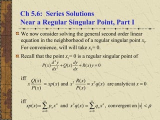
Our differential equation has the form
Dividing by P(x) and multiplying by x2
, we obtain
Substituting in the power series representations of p and q,
we obtain
0)()()( =+′+′′ yxRyxQyxP
∑∑
∞
=
∞
=
==
0
2
0
,)(,)(
n
n
n
n
n
n xqxqxxpxxp
[ ] [ ] 0)()( 22
=+′+′′ yxqxyxxpxyx
( ) ( ) 02
210
2
210
2
=++++′++++′′ yxqxqqyxpxppxyx ](data:image/gif;base64,R0lGODlhAQABAIAAAAAAAP///yH5BAEAAAAALAAAAAABAAEAAAIBRAA7)
Empfohlen
Weitere ähnliche Inhalte
Was ist angesagt?
Was ist angesagt? (20)
Ähnlich wie Ch05 6
Ähnlich wie Ch05 6 (20)
Ch05 6
- 1. Ch 5.6: Series Solutions Near a Regular Singular Point, Part I We now consider solving the general second order linear equation in the neighborhood of a regular singular point x0. For convenience, will will take x0= 0. Recall that the point x0= 0 is a regular singular point of iff iff 0)()()( 2 2 =++ yxR dx dy xQ dx yd xP 0atanalyticare)( )( )( and)( )( )( 22 === xxqx xP xR xxxp xP xQ x onconvergent,)(and)( 0 2 0 ρ<== ∑∑ ∞ = ∞ = n n n n n n xxqxqxxpxxp
- 2. Transforming Differential Equation Our differential equation has the form Dividing by P(x) and multiplying by x2 , we obtain Substituting in the power series representations of p and q, we obtain 0)()()( =+′+′′ yxRyxQyxP ∑∑ ∞ = ∞ = == 0 2 0 ,)(,)( n n n n n n xqxqxxpxxp [ ] [ ] 0)()( 22 =+′+′′ yxqxyxxpxyx ( ) ( ) 02 210 2 210 2 =++++′++++′′ yxqxqqyxpxppxyx
- 3. Comparison with Euler Equations Our differential equation now has the form Note that if then our differential equation reduces to the Euler Equation In any case, our equation is similar to an Euler Equation but with power series coefficients. Thus our solution method: assume solutions have the form ( ) 0,0for,)( 0 0 2 210 ∑ ∞ = + >≠=+++= n nr n r xaxaxaxaaxxy ( ) ( ) 02 210 2 210 2 =++++′++++′′ yxqxqqyxpxppxyx 02121 ====== qqpp 000 2 =+′+′′ yqyxpyx
- 4. Example 1: Regular Singular Point (1 of 13) Consider the differential equation This equation can be rewritten as Since the coefficients are polynomials, it follows that x = 0 is a regular singular point, since both limits below are finite: ( ) 012 2 =++′−′′ yxyxyx 0 2 1 2 2 = + +′−′′ y x y x yx ∞<= + ∞<−= − →→ 2 1 2 1 limand 2 1 2 lim 2 2 020 x x x x x x xx
- 5. Example 1: Euler Equation (2 of 13) Now xp(x) = -1/2 and x2 q(x) = (1 + x )/2, and thus for it follows that Thus the corresponding Euler Equation is As in Section 5.5, we obtain We will refer to this result later. 0,2/1,2/1,2/1 3221100 ========−= qqppqqp ∑∑ ∞ = ∞ = == 0 2 0 ,)(,)( n n n n n n xqxqxxpxxp 020 2 00 2 =+′−′′⇔=+′+′′ yyxyxyqyxpyx [ ] ( )( ) 2/1,1011201)1(2 ==⇔=−−⇔=+−− rrrrrrrxr ( ) 012 2 =++′−′′ yxyxyx
- 6. Example 1: Differential Equation (3 of 13) For our differential equation, we assume a solution of the form By substitution, our differential equation becomes or ( ) 012 2 =++′−′′ yxyxyx ( ) ( )( )∑ ∑ ∑ ∞ = −+ ∞ = ∞ = −++ −++=′′ +=′= 0 2 0 0 1 1)( ,)(,)( n nr n n n nr n nr n xnrnraxy xnraxyxaxy ( )( ) ( ) 012 0 1 000 =+++−−++ ∑∑∑∑ ∞ = ++ ∞ = + ∞ = + ∞ = + n nr n n nr n n nr n n nr n xaxaxnraxnrnra ( )( ) ( ) 012 1 1 000 =+++−−++ ∑∑∑∑ ∞ = + − ∞ = + ∞ = + ∞ = + n nr n n nr n n nr n n nr n xaxaxnraxnrnra
- 7. Example 1: Combining Series (4 of 13) Our equation can next be written as It follows that and ( )( ) ( ) 012 1 1 000 =+++−−++ ∑∑∑∑ ∞ = + − ∞ = + ∞ = + ∞ = + n nr n n nr n n nr n n nr n xaxaxnraxnrnra [ ] ( )( )[ ]{ } 01)(121)1(2 1 10 =+++−−++++−− ∑ ∞ = + − n nr nn r xanrnrnraxrrra [ ] 01)1(20 =+−− rrra ( )( )[ ] ,2,1,01)(12 1 ==+++−−++ − nanrnrnra nn
- 8. Example 1: Indicial Equation (5 of 13) From the previous slide, we have The equation is called the indicial equation, and was obtained earlier when we examined the corresponding Euler Equation. The roots r1= 1, r2 = ½, of the indicial equation are called the exponents of the singularity, for regular singular point x = 0. The exponents of the singularity determine the qualitative behavior of solution in neighborhood of regular singular point. [ ] 0)1)(12(13201)1(2 2 0 0 0 =−−=+−⇔=+−− ≠ rrrrrrra a [ ] ( )( )[ ]{ } 01)(121)1(2 1 10 =+++−−++++−− ∑ ∞ = + − n nr nn r xanrnrnraxrrra
- 9. Example 1: Recursion Relation (6 of 13) Recall that We now work with the coefficient on xr+n : It follows that [ ] ( )( )[ ]{ } 01)(121)1(2 1 10 =+++−−++++−− ∑ ∞ = + − n nr nn r xanrnrnraxrrra ( )( )[ ] 01)(12 1 =+++−−++ −nn anrnrnra ( )( ) ( ) ( )[ ] ( )[ ] 1, 112 1)(32 1)(12 1 2 1 1 ≥ −+−+ −= ++−+ −= ++−−++ −= − − − n nrnr a nrnr a nrnrnr a a n n n n
- 10. Example 1: First Root (7 of 13) We have Starting with r1= 1, this recursion becomes Thus ( )[ ] ( )[ ] 2/1and1,1for, 112 11 1 ==≥ −+−+ −= − rrn nrnr a a n n ( )[ ] ( )[ ] ( ) 1, 1211112 11 ≥ + −= −+−+ −= −− n nn a nn a a nn n ( )( )215325 13 01 2 0 1 ⋅⋅ = ⋅ −= ⋅ −= aa a a a ( )( ) ( )( ) 1, !12753 )1( etc, 32175337 0 02 3 ≥ +⋅⋅ − = ⋅⋅⋅⋅ −= ⋅ −= n nn a a aa a n n
- 11. Example 1: First Solution (8 of 13) Thus we have an expression for the n-th term: Hence for x > 0, one solution to our differential equation is ( )( ) 1, !12753 )1( 0 ≥ +⋅⋅ − = n nn a a n n ( )( ) ( )( ) +⋅⋅ − += +⋅⋅ − += = ∑ ∑ ∑ ∞ = ∞ = + + ∞ = 1 0 1 1 0 0 0 1 !12753 )1( 1 !12753 )1( )( n nn n nn rn n n nn x xa nn xa xa xaxy
- 12. Example 1: Radius of Convergence for First Solution (9 of 13) Thus if we omit a0, one solution of our differential equation is To determine the radius of convergence, use the ratio test: Thus the radius of convergence is infinite, and hence the series converges for all x. ( )( ) 0, !12753 )1( 1)( 1 1 > +⋅⋅ − += ∑ ∞ = x nn x xxy n nn ( )( ) ( )( )( )( ) ( )( ) 10 132 lim )1(!13212753 )1(!12753 limlim 111 1 <= ++ = −+++⋅⋅ −+⋅⋅ = ∞→ ++ ∞→ + + ∞→ nn x xnnn xnn xa xa n nn nn nn n n n n
- 13. Example 1: Second Root (10 of 13) Recall that When r1= 1/2, this recursion becomes Thus ( )[ ] ( )[ ] 2/1and1,1for, 112 11 1 ==≥ −+−+ −= − rrn nrnr a a n n ( )[ ] ( )[ ] ( ) ( ) 1, 122/1212/112/12 111 ≥ − −= − −= −+−+ −= −−− n nn a nn a nn a a nnn n ( )( )312132 11 01 2 0 1 ⋅⋅ = ⋅ −= ⋅ −= aa a a a ( )( ) ( ) ( )( ) 1, !12531 )1( etc, 53132153 0 02 3 ≥ −⋅⋅ − = ⋅⋅⋅⋅ −= ⋅ −= n nn a a aa a n n
- 14. Example 1: Second Solution (11 of 13) Thus we have an expression for the n-th term: Hence for x > 0, a second solution to our equation is ( )( ) 1, !12531 )1( 0 ≥ −⋅⋅ − = n nn a a n n ( )( ) ( )( ) −⋅⋅ − += −⋅⋅ − += = ∑ ∑ ∑ ∞ = ∞ = + + ∞ = 1 2/1 0 1 2/1 02/1 0 0 2 !12531 )1( 1 !12531 )1( )( n nn n nn rn n n nn x xa nn xa xa xaxy
- 15. Example 1: Radius of Convergence for Second Solution (12 of 13) Thus if we omit a0, the second solution is To determine the radius of convergence for this series, we can use the ratio test: Thus the radius of convergence is infinite, and hence the series converges for all x. ( )( ) ( )( )( )( ) ( ) 10 12 lim )1(!11212531 )1(!12531 limlim 111 1 <= + = −++−⋅⋅ −−⋅⋅ = ∞→ ++ ∞→ + + ∞→ nn x xnnn xnn xa xa n nn nn nn n n n n ( )( ) −⋅⋅ − += ∑ ∞ =1 2/1 2 !12531 )1( 1)( n nn nn x xxy
- 16. Example 1: General Solution (13 of 13) The two solutions to our differential equation are Since the leading terms of y1 and y2 are x and x1/2 , respectively, it follows that y1 and y2 are linearly independent, and hence form a fundamental set of solutions for differential equation. Therefore the general solution of the differential equation is where y1 and y2 are as given above. ( )( ) ( )( ) −⋅⋅ − += +⋅⋅ − += ∑ ∑ ∞ = ∞ = 1 2/1 2 1 1 !12531 )1( 1)( !12753 )1( 1)( n nn n nn nn x xxy nn x xxy ,0),()()( 2211 >+= xxycxycxy
- 17. Shifted Expansions & Discussion For the analysis given in this section, we focused on x = 0 as the regular singular point. In the more general case of a singular point at x = x0, our series solution will have the form If the roots r1, r2 of the indicial equation are equal or differ by an integer, then the second solution y2 normally has a more complicated structure. These cases are discussed in Section 5.7. If the roots of the indicial equation are complex, then there are always two solutions with the above form. These solutions are complex valued, but we can obtain real-valued solutions from ( ) ( )n n n r xxaxxxy 0 0 0)( −−= ∑ ∞ =