SlideShare ist ein Scribd-Unternehmen logo
1 von 55
Downloaden Sie, um offline zu lesen
See how recursive functions and structural induction relate to recursive datatypes
Follow along as the fold abstraction is introduced and explained
Watch as folding is used to simplify the definition of recursive functions over recursive datatypes
Part 1 - through the work of
Folding Unfolded
Polyglot FP for Fun and Profit
Haskell and Scala
Graham Hutton
@haskellhutt
@philip_schwarzslides by https://www.slideshare.net/pjschwarz
Richard Bird
http://www.cs.ox.ac.uk/people/richard.bird/
Richard Bird
@philip_schwarz
This slide deck is almost entirely centered on material from Richard Bird’s fantastic book, Introduction to Functional
Programming using Haskell.
I hope he’ll forgive me for relying so heavily on his work, but I couldn’t resist using extensive excerpts from his compelling book
to introduce and explain the concept of folding.
http://www.cs.ox.ac.uk/people/richard.bird/
https://en.wikipedia.org/wiki/Richard_Bird_(computer_scientist)
3.1 Natural Numbers
The natural numbers are the numbers 0, 1, 2 and so on, used for counting. The type 𝑵𝒂𝒕 is introduced by the declaration
𝐝𝐚𝐭𝐚 𝑵𝒂𝒕 = 𝒁𝒆𝒓𝒐 | 𝑺𝒖𝒄𝒄 𝑵𝒂𝒕
𝑵𝒂𝒕 is our first example of a recursive datatype declaration. The definition says that Zero is a value of 𝑵𝒂𝒕, and that Succ 𝑛 is a
value of 𝑵𝒂𝒕 whenever 𝑛 is. In particular, the constructor 𝑺𝒖𝒄𝒄 (short for ‘successor’), has type 𝑵𝒂𝒕 → 𝑵𝒂𝒕. For example, each of
𝒁𝒆𝒓𝒐, 𝑺𝒖𝒄𝒄 𝒁𝒆𝒓𝒐, 𝑺𝒖𝒄𝒄 (𝑺𝒖𝒄𝒄 𝒁𝒆𝒓𝒐)
is an element of 𝑵𝒂𝒕. As an element of 𝑵𝒂𝒕 the number 7 would be represented by
𝑺𝒖𝒄𝒄 (𝑺𝒖𝒄𝒄 (𝑺𝒖𝒄𝒄 (𝑺𝒖𝒄𝒄 (𝑺𝒖𝒄𝒄 (𝑺𝒖𝒄𝒄 (𝑺𝒖𝒄𝒄 𝒁𝒆𝒓𝒐))))))
Every natural number is represented by a unique value of 𝑵𝒂𝒕. On the other hand, not every value of 𝑵𝒂𝒕 represents a well-
defined natural number. In fact 𝑵𝒂𝒕 also contains the values ⊥, 𝑺𝒖𝒄𝒄 ⊥, 𝑺𝒖𝒄𝒄 (𝑺𝒖𝒄𝒄 ⊥), and so on. These additional values will
be discussed later.
Let us see how to program the basic arithmetic and comparison operations on 𝑵𝒂𝒕. Addition can be defined by
+ ∷ 𝑵𝒂𝒕 → 𝑵𝒂𝒕 → 𝑵𝒂𝒕
𝑚 + 𝒁𝒆𝒓𝒐 = 𝑚
𝑚 + 𝑺𝒖𝒄𝒄 𝑛 = 𝑺𝒖𝒄𝒄 𝑚 + 𝑛
This is a recursive definition, defining + by pattern matching on the second argument. Since every element of 𝑵𝒂𝒕, apart for ⊥, is
either 𝒁𝒆𝒓𝒐 or of the form Succ 𝑛, where 𝑛 is an element of 𝑵𝒂𝒕, the two patterns in the equations for + are disjoint and cover all
numbers apart from ⊥.

 Richard Bird
Here is how 𝒁𝒆𝒓𝒐 + 𝑺𝒖𝒄𝒄 (𝑺𝒖𝒄𝒄 𝒁𝒆𝒓𝒐) would be evaluated:
𝒁𝒆𝒓𝒐 + 𝑺𝒖𝒄𝒄 (𝑺𝒖𝒄𝒄 𝒁𝒆𝒓𝒐)
= { second equation for +, i.e. 𝑚 + 𝑺𝒖𝒄𝒄 𝑛 = 𝑺𝒖𝒄𝒄 𝑚 + 𝑛 }
𝑺𝒖𝒄𝒄 𝒁𝒆𝒓𝒐 + 𝑺𝒖𝒄𝒄 𝒁𝒆𝒓𝒐
= { second equation for +, i.e. 𝑚 + 𝑺𝒖𝒄𝒄 𝑛 = 𝑺𝒖𝒄𝒄 𝑚 + 𝑛 }
𝑺𝒖𝒄𝒄 𝑺𝒖𝒄𝒄 (𝒁𝒆𝒓𝒐 + 𝒁𝒆𝒓𝒐)
= { first equation for +, i.e. 𝑚 + 𝒁𝒆𝒓𝒐 = 𝑚 }
𝑺𝒖𝒄𝒄 (𝑺𝒖𝒄𝒄 𝒁𝒆𝒓𝒐)

it is not a practical proposition to introduce natural numbers through the datatype 𝑵𝒂𝒕: arithmetic would be just too inefficient.
In particular, calculating 𝑚 + n would require (𝑛 + 1) evaluation steps. On the other hand, counting on your fingers is a good way
to understand addition.
Given +, we can define ×:
(×) ∷ 𝑵𝒂𝒕 → 𝑵𝒂𝒕 → 𝑵𝒂𝒕
𝑚 × 𝒁𝒆𝒓𝒐 = 𝒁𝒆𝒓𝒐
𝑚 × 𝑺𝒖𝒄𝒄 𝑛 = 𝑚 × 𝑛 + 𝑚
Given ×, we can define exponentiation (↑) by
(↑) ∷ 𝑵𝒂𝒕 → 𝑵𝒂𝒕 → 𝑵𝒂𝒕
𝑚 ↑ 𝒁𝒆𝒓𝒐 = 𝑺𝒖𝒄𝒄 𝒁𝒆𝒓𝒐
𝑚 ↑ 𝑺𝒖𝒄𝒄 𝑛 = 𝑚 ↑ 𝑛 × 𝑚


Richard Bird
On the next slide we show the definitions of +, ×,
and ↑ again, and have a go at implementing the
three operations in Scala, together with some tests.
val `(+)`: Nat => Nat => Nat =
m => {
case Zero => m
case Succ(n) => Succ(m + n)
}
implicit class NatOps(m: Nat){
def +(n: Nat) = `(+)`(m)(n)
def ×(n: Nat) = `(×)`(m)(n)
def ↑(n: Nat) = `(↑)`(m)(n)
}
sealed trait Nat
case class Succ(n: Nat) extends Nat
case object Zero extends Nat
+ ∷ 𝑵𝒂𝒕 → 𝑵𝒂𝒕 → 𝑵𝒂𝒕
𝑚 + 𝒁𝒆𝒓𝒐 = 𝑚
𝑚 + 𝑺𝒖𝒄𝒄 𝑛 = 𝑺𝒖𝒄𝒄 𝑚 + 𝑛
val `(×)`: Nat => Nat => Nat =
m => {
case Zero => Zero
case Succ(n) => (m × n) + m
}
val `(↑)`: Nat => Nat => Nat =
m => {
case Zero => Succ(Zero)
case Succ(n) => (m ↑ n) × m
}
(×) ∷ 𝑵𝒂𝒕 → 𝑵𝒂𝒕 → 𝑵𝒂𝒕
𝑚 × 𝒁𝒆𝒓𝒐 = 𝒁𝒆𝒓𝒐
𝑚 × 𝑺𝒖𝒄𝒄 𝑛 = 𝑚 × 𝑛 + 𝑚
(↑) ∷ 𝑵𝒂𝒕 → 𝑵𝒂𝒕 → 𝑵𝒂𝒕
𝑚 ↑ 𝒁𝒆𝒓𝒐 = 𝑺𝒖𝒄𝒄 𝒁𝒆𝒓𝒐
𝑚 ↑ 𝑺𝒖𝒄𝒄 𝑛 = 𝑚 ↑ 𝑛 × 𝑚
𝐝𝐚𝐭𝐚 𝑵𝒂𝒕 = 𝒁𝒆𝒓𝒐 | 𝑺𝒖𝒄𝒄 𝑵𝒂𝒕
; assert(0 + 0 == 0) ; assert(Zero + Zero == Zero)
; assert(0 + 1 == 1) ; assert(Zero + Succ(Zero) == Succ(Zero))
; assert(1 + 0 == 1) ; assert(Succ(Zero) + Zero == Succ(Zero))
; assert(1 + 1 == 2) ; assert(Succ(Zero) + Succ(Zero) == Succ(Succ(Zero)))
; assert(2 + 3 == 5) ; assert(Succ(Succ(Zero)) + Succ(Succ(Succ(Zero))) == Succ(Succ(Succ(Succ(Succ(Zero))))))
; assert(0 * 0 == 0) ; assert((Zero × Zero) == Zero)
; assert(1 * 0 == 0) ; assert((Succ(Zero) × Zero) == Zero)
; assert(0 * 1 == 0) ; assert((Zero × Succ(Zero)) == Zero)
; assert(1 * 1 == 1) ; assert((Succ(Zero) × Succ(Zero)) == Succ(Zero))
; assert(1 * 2 == 2) ; assert((Succ(Zero) × Succ(Succ(Zero))) == Succ(Succ(Zero)))
; assert(2 * 3 == 6) ; assert((Succ(Succ(Zero)) × Succ(Succ(Succ(Zero)))) == Succ(Succ(Succ(Succ(Succ(Succ(Zero)))))))
; assert(Math.pow(1,0) == 1) ; assert( (Succ(Zero) ↑ Zero) == Succ(Zero) )
; assert(Math.pow(2,2) == 4) ; assert( (Succ(Succ(Zero)) ↑ Succ(Succ(Zero))) == Succ(Succ(Succ(Succ(Zero)))) )
The remaining arithmetic operation common to all numbers is subtraction (−). However, subtraction is a partial operation on
natural numbers. The definition is
− ∷ 𝑵𝒂𝒕 → 𝑵𝒂𝒕 → 𝑵𝒂𝒕
𝑚 − 𝒁𝒆𝒓𝒐 = 𝑚
𝑺𝒖𝒄𝒄 𝑚 − 𝑺𝒖𝒄𝒄 𝑛 = 𝑚 − 𝑛
This definition uses pattern matching on both arguments; taken together, the patterns are disjoint but not exhaustive. For
example,
𝑺𝒖𝒄𝒄 𝒁𝒆𝒓𝒐 − 𝑺𝒖𝒄𝒄 (𝑺𝒖𝒄𝒄 𝒁𝒆𝒓𝒐)
= { second equation for −, i.e. 𝑺𝒖𝒄𝒄 𝑚 − 𝑺𝒖𝒄𝒄 𝑛 = 𝑚 − 𝑛 }
𝒁𝒆𝒓𝒐 − 𝑺𝒖𝒄𝒄 𝒁𝒆𝒓𝒐
= { case exhaustion }
⊥
The hint ‘case exhaustion’ in the last step indicates that no equation for − has a pattern that matches (𝒁𝒆𝒓𝒐 − 𝑺𝒖𝒄𝒄 𝒁𝒆𝒓𝒐).
More generally, 𝑚 − 𝑛 = ⊥ if 𝑚 < 𝑛. The partial nature of subtraction on the natural numbers is the prime motivation for
introducing the integer numbers; over the integers, − is a total operation.
...Finally, here are two more examples of programming with 𝑵𝒂𝒕. The factorial and Fibonacci functions are defined by
𝑓𝑎𝑐𝑡 ∷ 𝑵𝒂𝒕 → 𝑵𝒂𝒕
𝑓𝑎𝑐𝑡 𝒁𝒆𝒓𝒐 = 𝑺𝒖𝒄𝒄 𝒁𝒆𝒓𝒐
𝑓𝑎𝑐𝑡 𝑺𝒖𝒄𝒄 𝑛 = 𝑺𝒖𝒄𝒄 𝑛 × 𝑓𝑎𝑐𝑡 𝑛
𝑓𝑖𝑏 ∷ 𝑵𝒂𝒕 → 𝑵𝒂𝒕
𝑓𝑖𝑏 𝒁𝒆𝒓𝒐 = 𝑺𝒖𝒄𝒄 𝒁𝒆𝒓𝒐
𝑓𝑖𝑏 𝑺𝒖𝒄𝒄 𝒁𝒆𝒓𝒐 = 𝑺𝒖𝒄𝒄 𝒁𝒆𝒓𝒐
𝑓𝑖𝑏 𝑺𝒖𝒄𝒄 𝑺𝒖𝒄𝒄 𝑛 = 𝑓𝑖𝑏 𝑺𝒖𝒄𝒄 𝑛 + 𝑓𝑖𝑏 𝑛 Richard Bird
See the next slide for a Scala
implementation of the − operation.
− ∷ 𝑵𝒂𝒕 → 𝑵𝒂𝒕 → 𝑵𝒂𝒕
𝑚 − 𝒁𝒆𝒓𝒐 = 𝑚
𝑺𝒖𝒄𝒄 𝑚 − 𝑺𝒖𝒄𝒄 𝑛 = 𝑚 − 𝑛
val `(-)`: Nat => Nat => Nat =
m => n => (m,n) match {
case (_,Zero) => m
case (Succ(x),Succ(y)) => x - y
}
; assert(0 - 0 == 0) ; assert(Zero - Zero == Zero)
; assert(1 - 0 == 1) ; assert(Succ(Zero) - Zero == Succ(Zero))
; assert(5 - 3 == 2) ; assert(Succ(Succ(Succ(Succ(Succ(Zero))))) - Succ(Succ(Succ(Zero))) == Succ(Succ(Zero)))
; assert(3 - 5 == -2) ; assert(
Try {
Succ(Succ(Succ(Zero))) - Succ(Succ(Succ(Succ(Succ(Zero)))))
}.toString.startsWith(
"Failure(scala.MatchError: (Zero,Succ(Succ(Zero)))"
)
)
No equation for − has a pattern that matches (𝒁𝒆𝒓𝒐 − 𝑺𝒖𝒄𝒄 𝒁𝒆𝒓𝒐).
Similarly for (𝒁𝒆𝒓𝒐 − 𝑺𝒖𝒄𝒄 (𝑺𝒖𝒄𝒄 𝒁𝒆𝒓𝒐)), (𝒁𝒆𝒓𝒐 − 𝑺𝒖𝒄𝒄 (𝑺𝒖𝒄𝒄(𝑺𝒖𝒄𝒄 𝒁𝒆𝒓𝒐))), etc.
More generally, 𝑚 − 𝑛 = ⊥ if 𝑚 < 𝑛.
𝑚 − 𝑛 throws scala.MatchError if 𝑚 < 𝑛.
@philip_schwarz
On the next slide we show the definitions of 𝑓𝑎𝑐𝑡,
and 𝑓𝑖𝑏 again, and have a go at implementing the
two functions in Scala, together with some tests.
val fact: Nat => Nat = {
case Zero => Succ(Zero)
case Succ(n) => Succ(n) × fact(n)
}
𝑓𝑎𝑐𝑡 ∷ 𝑵𝒂𝒕 → 𝑵𝒂𝒕
𝑓𝑎𝑐𝑡 𝒁𝒆𝒓𝒐 = 𝑺𝒖𝒄𝒄 𝒁𝒆𝒓𝒐
𝑓𝑎𝑐𝑡 𝑺𝒖𝒄𝒄 𝑛 = 𝑺𝒖𝒄𝒄 𝑛 × 𝑓𝑎𝑐𝑡 𝑛
𝑓𝑖𝑏 ∷ 𝑵𝒂𝒕 → 𝑵𝒂𝒕
𝑓𝑖𝑏 𝒁𝒆𝒓𝒐 = 𝑺𝒖𝒄𝒄 𝒁𝒆𝒓𝒐
𝑓𝑖𝑏 𝑺𝒖𝒄𝒄 𝒁𝒆𝒓𝒐 = 𝑺𝒖𝒄𝒄 𝒁𝒆𝒓𝒐
𝑓𝑖𝑏 𝑺𝒖𝒄𝒄 𝑺𝒖𝒄𝒄 𝑛 = 𝑓𝑖𝑏 𝑺𝒖𝒄𝒄 𝑛 + 𝑓𝑖𝑏 𝑛
val fib: Nat => Nat = {
case Zero => Succ(Zero)
case Succ(Zero) => Succ(Zero)
case Succ(Succ(n)) => fib(Succ(n)) + fib(n)
}
def factorial(n: Int): Int =
if (n == 0) 1
else n * factorial(n-1)
; assert(factorial(0) == 1) ; assert(fact(Zero) == Succ(Zero))
; assert(factorial(1) == 1) ; assert(fact(Succ(Zero)) == Succ(Zero))
; assert(factorial(2) == 2) ; assert(fact(Succ(Succ(Zero))) == Succ(Succ(Zero)))
; assert(factorial(3) == 6) ; assert(fact(Succ(Succ(Succ(Zero)))) == Succ(Succ(Succ(Succ(Succ(Succ(Zero)))))))
def fibonacci(n: Int): Int =
if (n == 0 || n == 1) 1
else fibonacci(n-1) + fibonacci(n-2)
; assert(fibonacci(0) == 1) ; assert(fib(Zero) == Succ(Zero))
; assert(fibonacci(1) == 1) ; assert(fib(Succ(Zero)) == Succ(Zero))
; assert(fibonacci(2) == 2) ; assert(fib(Succ(Succ(Zero))) == Succ(Succ(Zero)))
; assert(fibonacci(3) == 3) ; assert(fib(Succ(Succ(Succ(Zero)))) == Succ(Succ(Succ(Zero))))
; assert(fibonacci(4) == 5) ; assert(fib(Succ(Succ(Succ(Succ(Zero))))) == Succ(Succ(Succ(Succ(Succ(Zero))))))
; assert(fibonacci(5) == 8) ; assert(fib(Succ(Succ(Succ(Succ(Succ(Zero)))))) == Succ(Succ(Succ(Succ(Succ(Succ(Succ(Succ(Zero)))))))))
3.1.1 Partial numbers
Let us now return to the point about there being extra values in 𝑵𝒂𝒕. The values
⊥, 𝑺𝒖𝒄𝒄 ⊥, 𝑺𝒖𝒄𝒄 (𝑺𝒖𝒄𝒄 ⊥), 

are all different and each is also a member of 𝑵𝒂𝒕. That they exist is a consequence of three facts:
i. ⊥ is an element of 𝑵𝒂𝒕 because every datatype declaration introduces at least one extra value, the undefined value of
the type.
ii. constructor functions of a datatype are assumed to be nonstrict
iii. 𝑺𝒖𝒄𝒄 𝑛 is an element of Nat, whenever 𝑛 is
To appreciate why these extra values are different from one another, suppose we define 𝑢𝑛𝑑𝑒𝑓𝑖𝑛𝑒𝑑 ∷ 𝑵𝒂𝒕 by the equation
𝑢𝑛𝑑𝑒𝑓𝑖𝑛𝑒𝑑 = 𝑢𝑛𝑑𝑒𝑓𝑖𝑛𝑒𝑑. Then
? 𝒁𝒆𝒓𝒐 < 𝑢𝑛𝑑𝑒𝑓𝑖𝑛𝑒𝑑
{Interrupted!}
? 𝒁𝒆𝒓𝒐 < 𝑺𝒖𝒄𝒄 𝑢𝑛𝑑𝑒𝑓𝑖𝑛𝑒𝑑
𝑇𝑟𝑢𝑒
? 𝑺𝒖𝒄𝒄 𝒁𝒆𝒓𝒐 < 𝑺𝒖𝒄𝒄 𝑢𝑛𝑑𝑒𝑓𝑖𝑛𝑒𝑑
{Interrupted!}
? 𝑺𝒖𝒄𝒄 𝒁𝒆𝒓𝒐 < 𝑺𝒖𝒄𝒄 (𝑺𝒖𝒄𝒄 𝑢𝑛𝑑𝑒𝑓𝑖𝑛𝑒𝑑)
𝑇𝑟𝑢𝑒
One can interpret the extra values in the following way: ⊥ corresponds to the natural number about which there is
absolutely no information; 𝑺𝒖𝒄𝒄 ⊥ to the natural number about which the only information is that it is greater than 𝒁𝒆𝒓𝒐;
𝑺𝒖𝒄𝒄 (𝑺𝒖𝒄𝒄 ⊥) to the natural number about which the only information is that it is greater than 𝑺𝒖𝒄𝒄 𝒁𝒆𝒓𝒐; and so on.
Richard Bird
There is also one further value of 𝑵𝒂𝒕, namely the ‘infinite’ number:
𝑺𝒖𝒄𝒄 (𝑺𝒖𝒄𝒄 (𝑺𝒖𝒄𝒄 (𝑺𝒖𝒄𝒄 
 )))
This number can be defined by
𝑖𝑛𝑓𝑖𝑛𝑖𝑡𝑊 ∷ 𝑵𝒂𝒕
𝑖𝑛𝑓𝑖𝑛𝑖𝑡𝑊 = 𝑺𝒖𝒄𝒄 𝑖𝑛𝑓𝑖𝑛𝑖𝑡𝑊
It is different from all the other numbers, because it is the only number 𝑥 for which 𝑺𝒖𝒄𝒄 𝑚 < 𝑥 returns 𝑻𝒓𝒖𝒆 for all finite
numbers 𝑚. In this sense, 𝑖𝑛𝑓𝑖𝑛𝑖𝑡𝑊 is the largest element of 𝑵𝒂𝒕. If we request the value of 𝑖𝑛𝑓𝑖𝑛𝑖𝑡𝑊, then we obtain
? 𝑖𝑛𝑓𝑖𝑛𝑖𝑡𝑊
𝑺𝒖𝒄𝒄 (𝑺𝒖𝒄𝒄 (𝑺𝒖𝒄𝒄 (𝑺𝒖𝒄𝒄 (𝑺𝒖𝒄𝒄 {𝐌𝑛𝑡𝑒𝑟𝑟𝑢𝑝𝑡𝑒𝑑!}
The number 𝑖𝑛𝑓𝑖𝑛𝑖𝑡𝑊 satisfies other properties, in particular 𝑛 + 𝑖𝑛𝑓𝑖𝑛𝑖𝑡𝑊 = 𝑖𝑛𝑓𝑖𝑛𝑖𝑡𝑊, for all numbers 𝑛. The dual equation
𝑖𝑛𝑓𝑖𝑛𝑖𝑡𝑊 + 𝑛 = 𝑖𝑛𝑓𝑖𝑛𝑖𝑡𝑊 holds only for finite numbers 𝑛. We will see how to prove assertions such as these in the next
section.
To summarise this discussion, we can divide the values of 𝑵𝒂𝒕 into three classes:
• The finite numbers, those that correspond to well-defined natural numbers.
• The partial numbers, ⊥, 𝑺𝒖𝒄𝒄 ⊥, and so on.
• The infinite numbers, of which there is just one, namely 𝑖𝑛𝑓𝑖𝑛𝑖𝑡𝑊.
We will see that this classification holds true of all recursive types. There will be the finite elements of the type, the partial
elements, and the infinite elements. Although the infinite natural number is not of much use, the same is not true of the
infinite values of other datatypes.

 Richard Bird
Note that when in this slide deck we mention the concepts of ⊥
and 𝑖𝑛𝑓𝑖𝑛𝑖𝑡𝑊, it is mainly in a Haskell context, as we did in the last
two slides. In particular, we won’t be modelling ⊥ and 𝑖𝑛𝑓𝑖𝑛𝑖𝑡𝑊 in
any of the Scala code you’ll see throughout the deck.
3.2 Induction
In order to reason about the properties of recursively defined functions over a recursive datatype, we can appeal to a principle of
structural induction. In the case of 𝑵𝒂𝒕, the principle of structural induction can be defined as follows: In order to show that some
property 𝑃(𝑛) holds for each finite number 𝑛 of 𝑵𝒂𝒕, it is sufficient to show:
Case (𝒁𝒆𝒓𝒐). That 𝑃(𝒁𝒆𝒓𝒐) holds.
Case (𝑺𝒖𝒄𝒄 𝑛). That if 𝑃(𝑛) holds, then 𝑃(𝑺𝒖𝒄𝒄 𝑛) holds also.
Induction is valid for the same reason that recursive definitions are valid: every finite number is either 𝒁𝒆𝒓𝒐 or of the form
𝑺𝒖𝒄𝒄 𝑛, where 𝑛 is a finite number. If we prove the first case, then we have shown that the property is true for 𝒁𝒆𝒓𝒐; If we also
prove the second case, then we have shown that the property is true for 𝑺𝒖𝒄𝒄 𝒁𝒆𝒓𝒐, since it is true for 𝒁𝒆𝒓𝒐. But now, by the
same argument, it is true for 𝑺𝒖𝒄𝒄 𝑺𝒖𝒄𝒄 𝒁𝒆𝒓𝒐 , and so on.
The principle needs to be extended if we want to assert that some proposition is true for all elements of 𝑵𝒂𝒕, but we postpone
discussion of this point for the following section.
As an example, let’s prove that 𝒁𝒆𝒓𝒐 + 𝑛 = 𝑛 for all finite numbers 𝑛. Recall that + is defined by
𝑚 + 𝒁𝒆𝒓𝒐 = 𝑚
𝑚 + 𝑺𝒖𝒄𝒄 𝑛 = 𝑺𝒖𝒄𝒄 𝑚 + 𝑛
The first equation asserts that 𝒁𝒆𝒓𝒐 is a right unit of +. In general, 𝑒 is a left unit of ⊕ if 𝑒 ⊕ 𝑥 = 𝑥 for all 𝑥, and a right unit
of 𝑥 if 𝑥 ⊕ 𝑒 = 𝑥 for all 𝑥. If 𝑒 is both a left unit and a right unit of an operator ⊕, then it is called the unit of ⊕. The
terminology is appropriate since only one value can be both a left and right unit. So, by proving that 𝒁𝒆𝒓𝒐 is a left unit , we
have proved that 𝒁𝒆𝒓𝒐 is the unit of +.
Richard Bird
Proof. The proof is by induction on 𝑛. More precisely, we take for 𝑃(𝑛) the assertion that 𝒁𝒆𝒓𝒐 + 𝑛 = 𝑛. This equation is
referred to as the induction hypothesis.
Case (𝒁𝒆𝒓𝒐). We have to show 𝒁𝒆𝒓𝒐 + 𝒁𝒆𝒓𝒐 = 𝒁𝒆𝒓𝒐, which is immediate from the first equation defining +.
Case (𝑺𝒖𝒄𝒄 𝑛). We have to show that 𝒁𝒆𝒓𝒐 + 𝑺𝒖𝒄𝒄 𝑛 = 𝑺𝒖𝒄𝒄 𝑛, which we do by simplifying the left-hand expression:
𝒁𝒆𝒓𝒐 + 𝑺𝒖𝒄𝒄 𝑛
= { second equation for +, i.e. 𝑚 + 𝑺𝒖𝒄𝒄 𝑛 = 𝑺𝒖𝒄𝒄 𝑚 + 𝑛 }
𝑺𝒖𝒄𝒄 (𝒁𝒆𝒓𝒐 + 𝑛)
= { induction hypothesis}
𝑺𝒖𝒄𝒄 𝑛
☐
This example shows the format we will use for inductive proofs, laying out each case separately and using a ☐ to mark the end.
The very last step made use of the induction hypothesis, which is allowed by the way induction works.


3.2.1 Full Induction
In the form given above, the induction principle for 𝑵𝒂𝒕 suffices only to prove properties of the finite members of 𝑵𝒂𝒕. If we
want to show that a property 𝑃 also hold for every partial number, then we have to prove three things:
Case (⊥). That 𝑃(⊥) holds.
Case (𝒁𝒆𝒓𝒐). That 𝑃(𝒁𝒆𝒓𝒐) holds.
Case (𝑺𝒖𝒄𝒄 𝑛). That if 𝑃(𝑛) holds, then 𝑃(𝑺𝒖𝒄𝒄 𝑛) holds also.
We can omit the second case, but then we can conclude only that 𝑃(𝑛) holds for every partial number. The reason the
principle is valid is that is that every partial number is either ⊥ or of the form 𝑺𝒖𝒄𝒄 𝑛 for some partial number 𝑛. Richard Bird
To illustrate, let us prove the somewhat counterintuitive result that 𝑚 + 𝑛 = 𝑛 for all numbers 𝑚 and all partial numbers 𝑛.
Proof. The proof is by partial number induction on 𝑛.
Case (⊥). The equation 𝑚 + ⊥ = ⊥ follows at once by case exhaustion in the definition of +. That is, ⊥ does not match either of
the patterns 𝒁𝒆𝒓𝒐 or 𝑺𝒖𝒄𝒄 𝑛.
Case (𝑺𝒖𝒄𝒄 𝑛). For the left-hand side, we reason
𝑚 + 𝑺𝒖𝒄𝒄 𝑛
= { second equation for +, i.e. 𝑚 + 𝑺𝒖𝒄𝒄 𝑛 = 𝑺𝒖𝒄𝒄 𝑚 + 𝑛 }
𝑺𝒖𝒄𝒄 (𝑚 + 𝑛)
= { induction hypothesis}
𝑺𝒖𝒄𝒄 𝑛
Since the right-hand side is also 𝑺𝒖𝒄𝒄 𝑛, we are done.
3.2.2 Program synthesis
In the proofs above we defined some functions and then used induction to prove a certain property. We can also view
induction as a way to synthesise definitions of functions so that they satisfy the properties we want.
Let us illustrate with a simple example. Suppose we specify subtraction of natural numbers by the condition
𝑚 + 𝑛 − 𝑛 = 𝑚
for all 𝑚 and 𝑛. The specification does not give a constructive definition of − , merely a property that it has to satisfy.
However, we can do an induction proof on 𝑛 of the equation above, but view the calculation as a way of generating a suitable
definition of − .
Richard Bird
Unlike previous proofs, we reason with the equation as a whole, since simplification of both sides independently is not
possible if we do not know what all the rules of simplification are.
Case (𝒁𝒆𝒓𝒐). We reason
𝑚 + 𝒁𝒆𝒓𝒐 − 𝒁𝒆𝒓𝒐 = 𝑚
≡ { first equation for +, i.e. 𝑚 + 𝒁𝒆𝒓𝒐 = 𝑚 }
𝑚 − 𝒁𝒆𝒓𝒐 = 𝑚
Hence we can take 𝑚 − 𝒁𝒆𝒓𝒐 = 𝑚 to satisfy the case. The symbol ≡ is used to separate steps of the calculation since we are
calculating with mathematical assertions, not with values of a datatype.
Case (𝑺𝒖𝒄𝒄 𝑛). We reason
𝑚 + 𝑺𝒖𝒄𝒄 𝑛 − 𝑺𝒖𝒄𝒄 𝑛 = 𝑚
≡ { second equation for +, i.e. 𝑚 + 𝑺𝒖𝒄𝒄 𝑛 = 𝑺𝒖𝒄𝒄 𝑚 + 𝑛 }
𝑺𝒖𝒄𝒄 𝑚 + 𝑛 − 𝑺𝒖𝒄𝒄 𝑛 = 𝑚
≡ { hypothesis 𝑚 + 𝑛 − 𝑛 = 𝑚}
𝑺𝒖𝒄𝒄 𝑚 + 𝑛 − 𝑺𝒖𝒄𝒄 𝑛 = 𝑚 + 𝑛 − 𝑛
Replacing 𝑚 + 𝑛 in the last equation by 𝑚, we can take 𝑺𝒖𝒄𝒄 𝑚 − 𝑺𝒖𝒄𝒄 𝑛 = 𝑚 − 𝑛 to satisfy the case. Hence we have derived
𝑚 − 𝒁𝒆𝒓𝒐 = 𝑚
𝑺𝒖𝒄𝒄 𝑚 − 𝑺𝒖𝒄𝒄 𝑛 = 𝑚 − 𝑛
This is the program for − seen earlier.
Richard Bird
After that look at structural induction, it is finally time to
see how Richard Bird introduces the concept of folding.
3.3 The fold function
Many of the recursive definitions seen so far have a common pattern, exemplified by the following definition of a function 𝑓:
𝑓 ∷ 𝑵𝒂𝒕 → 𝐎
𝑓 𝒁𝒆𝒓𝒐 = 𝑐
𝑓 𝑺𝒖𝒄𝒄 𝑛 = ℎ 𝑓 𝑛
Here,	𝐎 is	some	type,	𝑐 is	an	element	of	𝐎,	and	ℎ ∷ 𝐎 → 𝐎 .	Observe	that	𝑓 works	by	taking	an	element	of	𝑵𝒂𝒕 and	replacing	
𝒁𝒆𝒓𝒐 by	𝑐 and	𝑺𝒖𝒄𝒄 by	ℎ.	For	example,	𝑓 takes	
𝑺𝒖𝒄𝒄 (𝑺𝒖𝒄𝒄 (𝑺𝒖𝒄𝒄 𝒁𝒆𝒓𝒐)) to				ℎ (ℎ (ℎ 𝑐))
The two equations for 𝑓 can be captured in terms of a single function, 𝑓𝑜𝑙𝑑𝑛, called the 𝑓𝑜𝑙𝑑 function for 𝑵𝒂𝒕. The definition is
𝑓𝑜𝑙𝑑𝑛 ∷ 𝛌 → 𝛌 → 𝛌 → 𝑵𝒂𝒕 → 𝛌
𝑓𝑜𝑙𝑑𝑛 ℎ 𝑐 𝒁𝒆𝒓𝒐 = 𝑐
𝑓𝑜𝑙𝑑𝑛 ℎ 𝑐 𝑺𝒖𝒄𝒄 𝑛 = ℎ 𝑓𝑜𝑙𝑑𝑛 ℎ 𝑐 𝑛
In	particular,	we have
𝑚 + 𝑛 = 𝑓𝑜𝑙𝑑𝑛 𝑺𝒖𝒄𝒄 𝑚 𝑛
𝑚 × 𝑛 = 𝑓𝑜𝑙𝑑𝑛 + 𝑚 𝒁𝒆𝒓𝒐 𝑛
𝑚 ↑ 𝑛 = 𝑓𝑜𝑙𝑑𝑛 × 𝑚 𝑺𝒖𝒄𝒄 𝒁𝒆𝒓𝒐 𝑛
It	follows	also	that	the	identity	function 𝑖𝑑 on	𝑵𝒂𝒕 satisfies 𝑖𝑑 = 𝑓𝑜𝑙𝑑𝑛 𝑺𝒖𝒄𝒄 𝒁𝒆𝒓𝒐. A suitable 𝑓𝑜𝑙𝑑 function can be defined for
every recursive type, and we will see other 𝑓𝑜𝑙𝑑 functions in the following chapters.
Richard Bird
+ ∷ 𝑵𝒂𝒕 → 𝑵𝒂𝒕 → 𝑵𝒂𝒕
𝑚 + 𝒁𝒆𝒓𝒐 = 𝑚
𝑚 + 𝑺𝒖𝒄𝒄 𝑛 = 𝑺𝒖𝒄𝒄 𝑚 + 𝑛
(×) ∷ 𝑵𝒂𝒕 → 𝑵𝒂𝒕 → 𝑵𝒂𝒕
𝑚 × 𝒁𝒆𝒓𝒐 = 𝒁𝒆𝒓𝒐
𝑚 × 𝑺𝒖𝒄𝒄 𝑛 = 𝑚 × 𝑛 + 𝑚
(↑) ∷ 𝑵𝒂𝒕 → 𝑵𝒂𝒕 → 𝑵𝒂𝒕
𝑚 ↑ 𝒁𝒆𝒓𝒐 = 𝑺𝒖𝒄𝒄 𝒁𝒆𝒓𝒐
𝑚 ↑ 𝑺𝒖𝒄𝒄 𝑛 = 𝑚 ↑ 𝑛 × 𝑚
+ ∷ 𝑵𝒂𝒕 → 𝑵𝒂𝒕 → 𝑵𝒂𝒕
𝑚 + 𝑛 = 𝑓𝑜𝑙𝑑𝑛 𝑺𝒖𝒄𝒄 𝑚 𝑛
(×) ∷ 𝑵𝒂𝒕 → 𝑵𝒂𝒕 → 𝑵𝒂𝒕
𝑚 × 𝑛 = 𝑓𝑜𝑙𝑑𝑛 + 𝑚 𝒁𝒆𝒓𝒐 𝑛
(↑) ∷ 𝑵𝒂𝒕 → 𝑵𝒂𝒕 → 𝑵𝒂𝒕
𝑚 ↑ 𝑛 = 𝑓𝑜𝑙𝑑𝑛 × 𝑚 𝑺𝒖𝒄𝒄 𝒁𝒆𝒓𝒐 𝑛
𝑓𝑜𝑙𝑑𝑛 ∷ 𝛌 → 𝛌 → 𝛌 → 𝑵𝒂𝒕 → 𝛌
𝑓𝑜𝑙𝑑𝑛 ℎ 𝑐 𝒁𝒆𝒓𝒐 = 𝑐
𝑓𝑜𝑙𝑑𝑛 ℎ 𝑐 𝑺𝒖𝒄𝒄 𝑛 = ℎ 𝑓𝑜𝑙𝑑𝑛 ℎ 𝑐 𝑛
@philip_schwarz
Just to reinforce the ideas on the previous slide, here are the original definitions
of +, × and ↑, and next to them, the new definitions in terms of 𝑓𝑜𝑙𝑑𝑛.
And the next slide is the same but in terms of Scala code.
val `(+)`: Nat => Nat => Nat =
m => {
case Zero => m
case Succ(n) => Succ(m + n)
}
val `(×)`: Nat => Nat => Nat =
m => {
case Zero => Zero
case Succ(n) => (m × n) + m
}
val `(↑)`: Nat => Nat => Nat =
m => {
case Zero => Succ(Zero)
case Succ(n) => (m ↑ n) × m
}
val `(×)`: Nat => Nat => Nat =
m => n => foldn((x:Nat) => x + m, Zero, n)
def foldn[A](h: A => A, c: A, n: Nat): A =
n match {
case Zero => c
case Succ(n) => h(foldn(h,c,n))
}
val `(↑)`: Nat => Nat => Nat =
m => n => foldn((x:Nat) => x × m, Succ(Zero), n)
val `(+)`: Nat => Nat => Nat =
m => n => foldn(Succ,m,n)
In	the	examples	above,	each	instance	of	𝑓𝑜𝑙𝑑𝑛 also	returned	an	element	of	𝑵𝒂𝒕.	In	the	following	two	examples,	𝑓𝑜𝑙𝑑𝑛
returns	an	element	of	(𝑵𝒂𝒕, 𝑵𝒂𝒕):
𝑓𝑎𝑐𝑡 ∷ 𝑵𝒂𝒕 → 𝑵𝒂𝒕
𝑓𝑎𝑐𝑡 = 𝑠𝑛𝑑 Š 𝑓𝑜𝑙𝑑𝑛 𝑓 (𝒁𝒆𝒓𝒐, 𝑺𝒖𝒄𝒄 𝒁𝒆𝒓𝒐)
where 𝑓 𝑚, 𝑛 = (𝑺𝒖𝒄𝒄 𝑚, 𝑺𝒖𝒄𝒄 (𝑚) × 𝑛)
𝑓𝑖𝑏 ∷ 𝑵𝒂𝒕 → 𝑵𝒂𝒕
𝑓𝑖𝑏 = 𝑓𝑠𝑡 Š 𝑓𝑜𝑙𝑑𝑛 𝑔 (𝒁𝒆𝒓𝒐, 𝑺𝒖𝒄𝒄 𝒁𝒆𝒓𝒐)
where 𝑔 𝑚, 𝑛 = (𝑛, 𝑚 + 𝑛)
The function 𝑓𝑎𝑐𝑡 computes the factorial function and function 𝑓𝑖𝑏 computes the Fibonacci function. Each program works by first
computing a more general result, namely an element of (𝑵𝒂𝒕, 𝑵𝒂𝒕), and then extracts the required result. In fact,
𝑓𝑜𝑙𝑑𝑛 𝑓 𝒁𝒆𝒓𝒐, 𝑺𝒖𝒄𝒄 𝒁𝒆𝒓𝒐 𝑛 = 𝑛, 𝑓𝑎𝑐𝑡 𝑛
𝑓𝑜𝑙𝑑𝑛 𝑔 𝒁𝒆𝒓𝒐, 𝑺𝒖𝒄𝒄 𝒁𝒆𝒓𝒐 𝑛 = 𝑓𝑖𝑏 𝑛, 𝑓𝑖𝑏 𝑺𝒖𝒄𝒄 𝑛
These equations can be proved by induction. The program for 𝑓𝑖𝑏 is more efficient than a direct recursive definition. The
recursive program requires an exponential number of + operations, while the program above requires only a linear number. We
will discuss efficiency in more detail in chapter 7, where the programming technique that led to the invention of the new program
for 𝑓𝑖𝑏 will be studied in a more general setting.
There are two advantages of writing recursive definitions in terms of 𝑓𝑜𝑙𝑑𝑛. Firstly, the definition is shorter; rather than having to
write down two equations, we have only to write down one. Secondly, it is possible to prove general properties of 𝑓𝑜𝑙𝑑𝑛 and use
them to prove properties of specific instantiations. In other words, rather than having to write down many induction proofs, we
have only to write down one.
Richard Bird
Now let’s have a very quick look at the
datatype for lists, and at induction over lists.
4.1.1 Lists as a datatype
A list can be constructed from scratch by starting with the empty list and successively adding elements one by one. One can add
elements to the front of the list, or to the rear, or to somewhere in the middle. In the following datatype declaration, nonempty
lists are constructed by adding elements to the front of the list:
𝐝𝐚𝐭𝐚 𝑳𝒊𝒔𝒕 𝛌 = 𝑵𝒊𝒍 | 𝑪𝒐𝒏𝒔 𝛌 (𝑳𝒊𝒔𝒕 𝛌)

The constructor (short for ‘construct’ – the name goes back to the programming language LISP) adds an element to the front of
the list. For example, the list 1,2,3 would be represented as the following element of 𝑳𝒊𝒔𝒕 𝑰𝒏𝒕:
𝑪𝒐𝒏𝒔 1 (𝑪𝒐𝒏𝒔 2 (𝑪𝒐𝒏𝒔 3 𝑵𝒊𝒍 ))
In functional programming, lists are defined as elements of 𝑳𝒊𝒔𝒕 𝛌. The syntax [𝛌] is used instead of 𝑳𝒊𝒔𝒕 𝛌, the constructor 𝑵𝒊𝒍 is
written as [ ], and the constructor 𝑪𝒐𝒏𝒔 is written as infix operator (∶). Moreover, (∶) associates to the right, so
1,2,3 = 1: 2: 3: [ ] = 1 ∶ 2 ∶ 3 ∶ [ ]
In other words, the special syntax on the left can be regarded as an abbreviation for the syntax on the right, which is also special,
but only by virtue of the fact that the constructors are given nonstandard names.
Like functions over other datatypes, functions over lists can be defined by pattern matching.
Richard Bird
Before moving on to the topic of induction over lists, Richard Bird gives
an example of a function defined over lists using pattern matching, but
the function he chooses is the equality function, whereas we are going
to choose the sum function, just to keep things simpler.
𝑠𝑢𝑚 ∷ [𝑰𝒏𝒕] → 𝑰𝒏𝒕
𝑠𝑢𝑚 [ ] = 0
𝑠𝑢𝑚 𝑥: 𝑥𝑠 = 𝑥 + (𝑠𝑢𝑚 𝑥𝑠)
val sum : List[Int] => Int = {
case Nil => 0
case x :: xs => x + sum(xs)
}
assert( sum( 4 :: (5 :: (6 :: Nil)) ) == 15)
sealed trait Nat
case class Succ(n: Nat) extends Nat
case object Zero extends Nat
sealed trait List[+A]
case class Cons[+A](head: A, tail: List[A]) extends List[A]
case object Nil extends List[Nothing]
val `(+)`: Nat => Nat => Nat =
m => { case Zero => m
case Succ(n) => Succ(m + n) }
implicit class NatSyntax(m: Nat){
def +(n: Nat) = `(+)`(m)(n)
}
val sum: List[Nat] => Nat = {
case Nil => Zero
case Cons(x, xs) => x + sum(xs)
}
assert( sum( Cons(
Succ(Zero), // 1
Cons(
Succ(Succ(Zero)), // 2
Cons(
Succ(Succ(Succ(Zero))), // 3
Nil))) )
== Succ(Succ(Succ(Succ(Succ(Succ(Zero))))))) // 6
𝑠𝑢𝑚 ∷ 𝑳𝒊𝒔𝒕 𝑵𝒂𝒕 → 𝑵𝒂𝒕
𝑠𝑢𝑚 𝑵𝒊𝒍 = 𝒁𝒆𝒓𝒐
𝑠𝑢𝑚 𝑪𝒐𝒏𝒔 𝑥 𝑥𝑠 = 𝑥 + (𝑠𝑢𝑚 𝑥𝑠)
+ ∷ 𝑵𝒂𝒕 → 𝑵𝒂𝒕 → 𝑵𝒂𝒕
𝑚 + 𝒁𝒆𝒓𝒐 = 𝑚
𝑚 + 𝑺𝒖𝒄𝒄 𝑛 = 𝑺𝒖𝒄𝒄 𝑚 + 𝑛
𝐝𝐚𝐭𝐚 𝑵𝒂𝒕 = 𝒁𝒆𝒓𝒐 | 𝑺𝒖𝒄𝒄 𝑵𝒂𝒕
𝐝𝐚𝐭𝐚 𝐋𝐢𝐬𝐭 α = 𝐍𝐢𝐥 | 𝐂𝐚𝐧𝐬 α (𝐋𝐢𝐬𝐭 α)
Same as on the previous slide, but this time
using Nat rather than Int, just for fun.
4.1.2 Induction over Lists
Recall from section 3.2 that, for the datatype 𝑵𝒂𝒕 of natural numbers, structural induction is based on three cases: every element
of 𝑵𝒂𝒕 is either ⊥, or 𝒁𝒆𝒓𝒐, or else has the form 𝑺𝒖𝒄𝒄 𝑛 for some element 𝑛 of 𝑵𝒂𝒕. Similarly, structural induction on lists is also
based on on three cases: every list is either the undefined list ⊥, the empty list [ ], or else has the form 𝑥: 𝑥𝑠 for some 𝑥 and list
𝑥𝑠.
To show by induction that a proposition 𝑃(𝑥𝑠) holds for all lists 𝑥𝑠 it suffices therefore to establish three cases:
Case (⊥). That 𝑃(⊥) holds.
Case ([ ]). That 𝑃([ ]) holds.
Case 𝑥: 𝑥𝑠 . That if 𝑃(𝑥𝑠) holds, then 𝑃(𝑥: 𝑥𝑠) also holds for every 𝑥.
If we prove only the second two cases, then we can conclude only that 𝑃(𝑥𝑠) holds for every finite list; if we prove only the first
and third cases. Then we can conclude only that 𝑃(𝑥𝑠) holds for every partial list. If 𝑃 takes the form of an equation, as all of our
laws do, then proving the first and third cases is sufficient to show that 𝑃(𝑥𝑠) holds for every infinite list. Partial lists and infinite
lists are described in the following section. Examples of induction proofs are given throughout the remainder of the chapter.
Richard Bird
Richard Bird provides other examples of recursive functions
over lists. Let’s see some of them: list concatenation,
flattening of lists of lists, list reversal and length of a list.
When looking at the first one, i.e. concatenation, let’s also
see an example of proof by structural induction on lists.
@philip_schwarz
4.2.1 Concatenation
Two lists can be concatenated to form one longer list. This function is denoted by the binary operator ⧺ (pronounced
‘concatenate’). As two simple examples, we have
? 1,2,3 ⧺ 4,5
1,2,3,4,5
? 1,2 ⧺ ⧺ 1
1,2,1
The formal definition of ⧺ is
(⧺) ∷ [α] → [α] → [α]
⧺ 𝑊𝑠 = 𝑊𝑠
𝑥: 𝑥𝑠 ⧺ 𝑊𝑠 = 𝑥 ∶ (𝑥𝑠 ⧺ 𝑊𝑠)
Concatenation takes two lists, both of the same type, and produces a third list, again of the same type. Hence the type assignment.
The definition of ⧺ is by pattern matching on the left-hand argument; the two patterns are disjoint and cover all cases, apart from
the undefined list ⊥. It follows by case exhaustion that ⊥ ⧺ 𝑊𝑠 = ⊥.
However, it is not the case that 𝑊𝑠 ⧺ ⊥ = ⊥. For example,
? 1,2,3 ⧺ 𝑢𝑛𝑑𝑒𝑓𝑖𝑛𝑒𝑑
1,2,3{𝐌𝑛𝑡𝑒𝑟𝑟𝑢𝑝𝑡𝑒𝑑!}
The list 1,2,3 ⧺ ⊥ is a partial list; In full form it is the list 1: 2: 3: ⊥. The evaluator can compute the first three elements, but
thereafter it goes into a nonterminating computation, so we interrupt it.
The second equation for ⧺ is very succinct and requires some thought. Once one has come to grips with the definition of ⧺, one Richard Bird
has understood a good deal about how lists work in functional programming. Note that the number of steps required to compute
𝑥𝑠 ⧺ 𝑊𝑠 is proportional to the number of elements in 𝑥𝑠.
1, 2 ⧺ 3, 4, 5
= { notation}
(1 ∶ 2 ∶ ⧺ (3 ∶ (4 ∶ 5 ∶ [ ] ))
= { second equation for ⧺, i.e. 𝑥: 𝑥𝑠 ⧺ 𝑊𝑠 = 𝑥 ∶ (𝑥𝑠 ⧺ 𝑊𝑠) }
1 ∶ ( 2 ∶ ⧺ (3 ∶ (4 ∶ 5 ∶ [ ] )))
= { second equation for ⧺ }
1 ∶ (2 ∶ ( ⧺ (3 ∶ (4 ∶ 5 ∶ [ ] ))))
= { first equation for ⧺ i.e. , ⧺ 𝑊𝑠 = 𝑊𝑠 }
1 ∶ (2 ∶ (3 ∶ (4 ∶ 5 ∶ [ ] )))
= { notation}
1, 2, 3, 4, 5
Concatenation is an associative operation with with unit :
𝑥𝑠 ⧺ 𝑊𝑠 ⧺ 𝑧𝑠 = 𝑥𝑠 ⧺ (𝑊𝑠 ⧺ 𝑧𝑠)
𝑥𝑠 ⧺ = ⧺ 𝑥𝑠 = 𝑥𝑠
Let us now prove by induction that ⧺ is associative.
Proof. The proof is by induction on 𝑥𝑠.
Case (⊥). For the left-hand side, we reason
⊥ ⧺ (𝑊𝑠 ⧺ 𝑧𝑠)
= { case exhaustion}
⊥ ⧺ 𝑧𝑠
= { case exhaustion}
⊥
Richard Bird
The right-hand side simplifies to ⊥ as well, establishing the case.
Case ([ ]). For the left hand side, we reason
[ ] ⧺ (𝑊𝑠 ⧺ 𝑧𝑠)
= { first equation for ⧺ i.e. , ⧺ 𝑊𝑠 = 𝑊𝑠 }
(𝑊𝑠 ⧺ 𝑧𝑠)
The right-hand side simplifies to(𝑊𝑠 ⧺ 𝑧𝑠) as well, establishing the case.
Case 𝑥 ∶ 𝑥𝑠 . For the left hand side, we reason
((x ∶ 𝑥𝑠) ⧺ 𝑊𝑠) ⧺ 𝑧𝑠
= { second equation for ⧺, i.e. 𝑥: 𝑥𝑠 ⧺ 𝑊𝑠 = 𝑥 ∶ (𝑥𝑠 ⧺ 𝑊𝑠) }
( 𝑥 ∶ 𝑥𝑠 ⧺ 𝑊𝑠) ⧺ 𝑧𝑠
= { second equation for ⧺ }
𝑥 ∶ ( 𝑥𝑠 ⧺ 𝑊𝑠 ⧺ 𝑧𝑠)
= { induction hypothesis }
𝑥 ∶ (𝑥𝑠 ⧺ 𝑊𝑠 ⧺ 𝑧𝑠)
For the right-hand side we reason
(x ∶ 𝑥𝑠) ⧺ (𝑊𝑠 ⧺ 𝑧𝑠)
= { second equation for ⧺, i.e. 𝑥 ∶ 𝑥𝑠 ⧺ 𝑊𝑠 = 𝑥 ∶ (𝑥𝑠 ⧺ 𝑊𝑠) }
𝑥 ∶ (𝑥𝑠 ⧺ (𝑊𝑠 ⧺ 𝑧𝑠))
The two sides are equal, establishing the case.

Note that associativity is proved for all lists, finite, partial or infinite. Hence we can assert that ⧺ is associative without
qualification
. Richard Bird
4.2.2 Concat
Concatenation performs much the same function for lists as the union operator ∪ does for sets. A companion function is concat,
which concatenates a list of lists into one long list. This function, which roughly corresponds to the big-union operator ⋃ for sets
of sets, is defined by
concat ∷ [ α ] → [α]
concat =
concat 𝑥𝑠: 𝑥𝑠𝑠 = 𝑥𝑠 ⧺ 𝑐𝑜𝑛𝑐𝑎𝑡 𝑥𝑠𝑠
For example,
?[ 1, 2 ⧺ ⧺ 3, 2,1 ]
1,2,3, 2,1
4.2.3 Reverse
Another basic function on lists is reverse, the function that reverses the order of elements in a finite list. For example:
? reverse “Madam, I’m Adam.”
“.MadA m’I ,madaM”
The definition is
reverse ∷ α → [α]
reverse =
reverse 𝑥 ∶ 𝑥𝑠 = 𝑟𝑒𝑣𝑒𝑟𝑠𝑒 𝑥𝑠 ⧺ [𝑥]
In words, to reverse a list 𝑥 ∶ 𝑥𝑠 , one reverses 𝑥𝑠, and then adds 𝑥 to the end. As a program, the above definition is not very Richard Bird
efficient: on a list of length 𝑛, it will need a number of reduction steps proportional to 𝑛2 to deliver the reversed list. The first
element will be appended to the end of a list of length 𝑛 − 1 , which will take about 𝑛 − 1 steps, the second element will be
appended to a list of length 𝑛 − 2 , taking 𝑛 − 2 steps, and so on. The total time is therefore about
𝑛 − 1 + 𝑛 − 2 + ⋯ 1 = 𝑛(𝑛 − 1)/2 steps
A more precise analysis is given in chapter 7, and a more efficient program for reverse is given in section 4.5.
4.2.2 Length
The length of a list is the number of elements it contains:
𝑙𝑒𝑛𝑔𝑡ℎ ∷ [α] → 𝑰𝒏𝒕
𝑙𝑒𝑛𝑔𝑡ℎ [ ] = 0
𝑙𝑒𝑛𝑔𝑡ℎ 𝑥: 𝑥𝑠 = 1 + 𝑙𝑒𝑛𝑔𝑡ℎ 𝑥𝑠
The nature of the list element is irrelevant when computing the length of a list, whence the type assignment. For example,
? 𝑙𝑒𝑛𝑔𝑡ℎ [𝑢𝑛𝑑𝑒𝑓𝑖𝑛𝑒𝑑, 𝑢𝑛𝑑𝑒𝑓𝑖𝑛𝑒𝑑]
2
However, not every list has a well-defined length. In particular, the partial lists ⊥, 𝑥 ∶ ⊥, 𝑥 ∶ 𝑊 ∶ ⊥, and so on, have an undefined
length. Only finite lists have well-defined lengths. The list ⊥, ⊥ is a finite list, not a partial list, because it is the list ⊥ ∶ ⊥ ∶ [ ],
which ends in [ ], not ⊥. The computer cannot produce the elements, but it can produce the length of the list.


Richard Bird
4.3 Map and filter
Two useful functions on lists are map and £ilter. The function map applies a function to each element of a list. For example
? 𝑚ap square [9, 3] ? 𝑚ap (<3) [1, 2, 3] ? 𝑚ap nextLetter “HAL”
[81, 9] [𝑇𝑟𝑢𝑒, 𝑇𝑟𝑢𝑒, 𝐹𝑎𝑙𝑠𝑒] “IBM”
The definition is
map ∷ (α → 𝛜) → [α] → [𝛜]
map f =
map f 𝑥 ∶ 𝑥𝑠 = 𝑓 𝑥 ∶ map 𝑓 𝑥𝑠


4.3 filter
The second function, filter, takes a Boolean function p and a list xs and returns that sublist of xs whose elements satisfy p. For
example,
? £ilter even [1,2,4,5,32] ? (sum Š map square Š £ilter even) [1. . 10]
[2,4,32] 220
The last example asks for the sum of the squares of the even integers in the range 1..10.
The definition of filter is
£ilter ∷ (α → 𝐵𝑜𝑜𝑙) → [α] → [α]
£ilter p =
£ilter p 𝑥 ∶ 𝑥𝑠 = 𝐢𝐟 𝑝 𝑥 𝐭𝐡𝐞𝐧 𝑥 ∶ £ilter p 𝑥𝑠 𝐞𝐥𝐬𝐞 £ilter p 𝑥𝑠

 Richard Bird
Now let’s look at fold functions over lists.
4.5 The fold functions
We have seen in the case of the datatype 𝑵𝒂𝒕 that many recursive definitions can be expressed very succinctly using a
suitable 𝑓𝑜𝑙𝑑 operator. Exactly the same is true of lists. Consider the following definition of a function ℎ :
ℎ [ ] = 𝑒
ℎ 𝑥: 𝑥𝑠 = 𝑥 ⊕ ℎ 𝑥𝑠
The function ℎ works by taking a list, replacing [ ] by 𝑒 and ∶ by ⊕, and evaluating the result. For example, ℎ converts the list
𝑥1 ∶ (𝑥2 ∶ 𝑥3 ∶ 𝑥4 ∶ )
to the value
𝑥1 ⊕ (𝑥2 ⊕ (𝑥3 ⊕ 𝑥4 ⊕ 𝑒 ))
Since ∶ associates to the right, there is no need to put in parentheses in the first expression. However, we do need to put in
parentheses in the second expression because we do not assume that ⊕ associates to the right.
The pattern of definition given by ℎ is captured in a function 𝑓𝑜𝑙𝑑𝑟 (prounced ‘fold right’) defined as follows:
𝑓𝑜𝑙𝑑𝑟 ∷ 𝛌 → 𝛜 → 𝛜 → 𝛜 → 𝛌 → 𝛜
𝑓𝑜𝑙𝑑𝑟 𝑓 𝑒 = 𝑒
𝑓𝑜𝑙𝑑𝑟 𝑓 𝑒 𝑥: 𝑥𝑠 = 𝑓 𝑥 𝑓𝑜𝑙𝑑𝑟 𝑓 𝑒 𝑥𝑠
We can now write h = 𝑓𝑜𝑙𝑑𝑟 ⊕ 𝑒. The first argument of 𝑓𝑜𝑙𝑑𝑟 is a binary operator that takes an 𝛌-value on its left and an a 𝛜–
value on its right, and delivers a 𝛜–value. The second argument of 𝑓𝑜𝑙𝑑𝑟 is a 𝛜-value. The third argument is of type 𝛌 , and the
result is of type 𝛜. In many cases, 𝛌 and 𝛜 will be instantiated to the same type, for instance when ⊕ denotes an associative
operation. Richard Bird
In the next slide we look at how some of the recursively
defined functions on lists that we have recently seen can be
redefined in terms of 𝑓𝑜𝑙𝑑𝑟.
To aid comprehension, I have added the original function
definitions next to the new definitions in terms of 𝑓𝑜𝑙𝑑𝑟. For
reference, I also added the definition of 𝑓𝑜𝑙𝑑𝑟.
The single function foldr can be used to define almost every function on lists that we have met so far. Here are just some
examples:
concat ∷ [ α ] → [α]
concat = 𝑓𝑜𝑙𝑑𝑟 (⧺) [ ]
reverse ∷ α → [α]
reverse = 𝑓𝑜𝑙𝑑𝑟 𝑠𝑛𝑜𝑐
𝑀ℎ𝑒𝑟𝑒 𝑠𝑛𝑜𝑐 𝑥 𝑥𝑠 = 𝑥𝑠 ⧺ [𝑥]
𝑙𝑒𝑛𝑔𝑡ℎ ∷ [α] → 𝑰𝒏𝒕
𝑙𝑒𝑛𝑔𝑡ℎ = 𝑓𝑜𝑙𝑑𝑟 𝑜𝑛𝑒𝑝𝑙𝑢𝑠 0
𝑀ℎ𝑒𝑟𝑒 𝑜𝑛𝑒𝑝𝑙𝑢𝑠 𝑥 𝑛 = 1 + 𝑛


𝑠𝑢𝑚 ∷ [𝑰𝒏𝒕] → 𝑰𝒏𝒕
𝑠𝑢𝑚 = 𝑓𝑜𝑙𝑑𝑟 + 0
map ∷ (α → 𝛜) → [α] → [𝛜]
map 𝑓 = 𝑓𝑜𝑙𝑑𝑟 𝑐𝑜𝑛𝑠 Š 𝑓
𝑀ℎ𝑒𝑟𝑒 𝑐𝑜𝑛𝑠 𝑥 𝑥𝑠 = 𝑥 ∶ 𝑥𝑠


concat ∷ [ α ] → [α]
concat =
concat 𝑥𝑠: 𝑥𝑠𝑠 = 𝑥𝑠 ⧺ 𝑐𝑜𝑛𝑐𝑎𝑡 𝑥𝑠𝑠
reverse ∷ α → [α]
reverse =
reverse 𝑥 ∶ 𝑥𝑠 = 𝑟𝑒𝑣𝑒𝑟𝑠𝑒 𝑥𝑠 ⧺ [𝑥]
𝑙𝑒𝑛𝑔𝑡ℎ ∷ [α] → 𝑰𝒏𝒕
𝑙𝑒𝑛𝑔𝑡ℎ [ ] = 0
𝑙𝑒𝑛𝑔𝑡ℎ 𝑥: 𝑥𝑠 = 1 + 𝑙𝑒𝑛𝑔𝑡ℎ 𝑥𝑠
𝑠𝑢𝑚 ∷ [𝑰𝒏𝒕] → 𝑰𝒏𝒕
𝑠𝑢𝑚 [ ] = 0
𝑠𝑢𝑚 𝑥: 𝑥𝑠 = 𝑥 + (𝑠𝑢𝑚 𝑥𝑠)
map ∷ (α → 𝛜) → [α] → [𝛜]
map f =
map f 𝑥 ∶ 𝑥𝑠 = 𝑓 𝑥 ∶ map 𝑓 𝑥𝑠
𝑓𝑜𝑙𝑑𝑟 ∷ 𝛌 → 𝛜 → 𝛜 → 𝛜 → 𝛌 → 𝛜
𝑓𝑜𝑙𝑑𝑟 𝑓 𝑒 = 𝑒
𝑓𝑜𝑙𝑑𝑟 𝑓 𝑒 𝑥: 𝑥𝑠 = 𝑓 𝑥 𝑓𝑜𝑙𝑑𝑟 𝑓 𝑒 𝑥𝑠 Richard Bird
On the next slide, the same code, translated into Scala
@philip_schwarz
def foldr[A,B](f: A => B => B)(e: B)(xs: List[A]): B =
xs match {
case Nil => e
case x::xs => f(x)(foldr(f)(e)(xs))
}
def concatenate[A]: List[A] => List[A] => List[A] =
xs => ys => xs match {
case Nil => ys
case x :: xs => x :: concatenate(xs)(ys)
}
def concat[A]: List[List[A]] => List[A] =
foldr(concatenate[A])(Nil)
def reverse[A]: List[A] => List[A] = {
def snoc[A]: A => List[A] => List[A] =
x => xs => concatenate(xs)(List(x))
foldr(snoc[A])(Nil)
}
def length[A]: List[A] => Int = {
def oneplus[A]: A => Int => Int = x => n => 1 + n
foldr(oneplus)(0)
}
val sum: List[Int] => Int = {
val plus: Int => Int => Int = a => b => a + b
foldr(plus)(0)
}
def map[A,B]: (A => B) => List[A] => List[B] = {
def cons: B => List[B] => List[B] = x => xs => x :: xs
f => foldr(cons compose f)(Nil)
}
𝑓𝑜𝑙𝑑𝑟 ∷ 𝛌 → 𝛜 → 𝛜 → 𝛜 → 𝛌 → 𝛜
𝑓𝑜𝑙𝑑𝑟 𝑓 𝑒 = 𝑒
𝑓𝑜𝑙𝑑𝑟 𝑓 𝑒 𝑥: 𝑥𝑠 = 𝑓 𝑥 𝑓𝑜𝑙𝑑𝑟 𝑓 𝑒 𝑥𝑠
(⧺) ∷ [α] → [α] → [α]
⧺ 𝑊𝑠 = 𝑊𝑠
𝑥: 𝑥𝑠 ⧺ 𝑊𝑠 = 𝑥 ∶ (𝑥𝑠 ⧺ 𝑊𝑠)
concat ∷ [ α ] → [α]
concat = 𝑓𝑜𝑙𝑑𝑟 (⧺) [ ]
reverse ∷ α → [α]
reverse = 𝑓𝑜𝑙𝑑𝑟 𝑠𝑛𝑜𝑐
𝑀ℎ𝑒𝑟𝑒 𝑠𝑛𝑜𝑐 𝑥 𝑥𝑠 = 𝑥𝑠 ⧺ [𝑥]
𝑙𝑒𝑛𝑔𝑡ℎ ∷ [α] → 𝑰𝒏𝒕
𝑙𝑒𝑛𝑔𝑡ℎ = 𝑓𝑜𝑙𝑑𝑟 𝑜𝑛𝑒𝑝𝑙𝑢𝑠 0
𝑀ℎ𝑒𝑟𝑒 𝑜𝑛𝑒𝑝𝑙𝑢𝑠 𝑥 𝑛 = 1 + 𝑛
𝑠𝑢𝑚 ∷ [𝑰𝒏𝒕] → 𝑰𝒏𝒕
𝑠𝑢𝑚 = 𝑓𝑜𝑙𝑑𝑟 + 0
map ∷ (α → 𝛜) → [α] → [𝛜]
map 𝑓 = 𝑓𝑜𝑙𝑑𝑟 𝑐𝑜𝑛𝑠 Q 𝑓
𝑀ℎ𝑒𝑟𝑒 𝑐𝑜𝑛𝑠 𝑥 𝑥𝑠 = 𝑥 ∶ 𝑥𝑠
assert( concatenate(List(1,2,3))(List(4,5)) == List(1,2,3,4,5) )
assert( concat(List(List(1,2), List(3), List(4,5))) == List(1,2,3,4,5) )
assert( reverse(List(1,2,3,4,5)) == List(5,4,3,2,1) )
assert( length(List(0,1,2,3,4,5)) == 6 )
assert( sum(List(2,3,4)) == 9 )
val mult: Int => Int => Int = a => b => a * b
assert( map(mult(10))(List(1,2,3)) == List(10,20,30))
Here a some sample tests for the
Scala functions on the previous slide.
It turns out that if it is possible to define a function on lists both using a recursive definition and
using a definition in terms of 𝑓𝑜𝑙𝑑𝑟, then there is a technique that can be used to go from the
recursive definition to the definition using 𝑓𝑜𝑙𝑑𝑟.
I came across the technique in the following paper by the author of Programming in Haskell:
The tutorial (which I shall be referring to as TUEF), shows how to apply the technique to the
sum function and the map function, which is the subject of the next five slides. Note: in the
paper, the 𝑓𝑜𝑙𝑑𝑟 function is referred to as 𝑓𝑜𝑙𝑑.
@philip_schwarz
3 The universal property of fold
As with the fold operator itself, the universal property of 𝒇𝒐𝒍𝒅 also has its origins in recursion theory. The first systematic use of the
universal property in functional programming was by Malcolm (1990a), in his generalisation of Bird and Meerten’s theory of lists (Bird,
1989; Meertens, 1983) to arbitrary regular datatypes. For finite lists, the universal property of 𝒇𝒐𝒍𝒅 can be stated as the following
equivalence between two definitions for a function 𝑔 that processes lists:
𝑔 = 𝑣 ⟺ 𝑔 = 𝑓𝑜𝑙𝑑 𝑓 𝑣
𝑔 𝑥 ∶ 𝑥𝑠 = 𝑓 𝑥 𝑔 𝑥𝑠
In the right-to-left direction, substituting 𝑔 = 𝑓𝑜𝑙𝑑 𝑓 𝑣 into the two equations for 𝑔 gives the recursive definition for 𝑓𝑜𝑙𝑑. Conversely,
in the left-to-right direction the two equations for g are precisely the assumptions required to show that 𝑔 = 𝑓𝑜𝑙𝑑 𝑓 𝑣 using a simple
proof by induction on finite lists (Bird, 1998). Taken as a whole, the universal property states that for finite lists the function 𝑓𝑜𝑙𝑑 𝑓 𝑣 is
not just a solution to its defining equations, but in fact the unique solution
. The universal property of 𝒇𝒐𝒍𝒅 can be generalised to
handle partial and infinite lists (Bird, 1998), but for simplicity we only consider finite lists in this article.
Graham Hutton
@haskellhutt
3.3 Universality as a definition principle
As well as being used as a proof principle, the universal property of 𝒇𝒐𝒍𝒅 can also be used as a definition principle that guides the
transformation of recursive functions into definitions using 𝑓𝑜𝑙𝑑. As a simple first example, consider the recursively defined function
𝑠𝑢𝑚 that calculates the sum of a list of numbers:
𝑠𝑢𝑚 ∷ 𝐌𝑛𝑡 → 𝐌𝑛𝑡
𝑠𝑢𝑚 = 0 𝑚
𝑠𝑢𝑚 𝑥 ∶ 𝑥𝑠 = 𝑥 + 𝑠𝑢𝑚 𝑥𝑠
Suppose now that we want to redefine 𝑠𝑢𝑚 using 𝑓𝑜𝑙𝑑. That is, we want to solve the equation 𝑠𝑢𝑚 = 𝑓𝑜𝑙𝑑 𝑓 𝑣 for a function f and a
value 𝑣. We begin by observing that the equation matches the right-hand side of the universal property, from which we conclude that
the equation is equivalent to the following two equations:
𝑠𝑢𝑚 = 𝑣
𝑠𝑢𝑚 𝑥 ∶ 𝑥𝑠 = 𝑓 𝑥 (𝑠𝑢𝑚 𝑥𝑠)
From the first equation and the definition of 𝑠𝑢𝑚, it is immediate that 𝑣 = 0.
𝑔 = 𝑣 ⟺ 𝑔 = 𝑓𝑜𝑙𝑑 𝑓 𝑣
𝑔 𝑥 ∶ 𝑥𝑠 = 𝑓 𝑥 𝑔 𝑥𝑠
Graham Hutton
@haskellhutt
From the second equation, we calculate a definition for f as follows:
𝑠𝑢𝑚 𝑥 ∶ 𝑥𝑠 = 𝑓 𝑥 (𝑠𝑢𝑚 𝑥𝑠)
⇔	 {	Definition	of	𝑠𝑢𝑚 }	
𝑥 + 𝑠𝑢𝑚 𝑥𝑠 = 𝑓 𝑥 (𝑠𝑢𝑚 𝑥𝑠)
⇐	 { †	Generalising	(𝑠𝑢𝑚 𝑥𝑠) to	𝑊 }	
𝑥 + 𝑊 = 𝑓 𝑥 𝑊
⇔	 {	Functions	}	
𝑓 = (+)
That is, using the universal property we have calculated that:
𝑠𝑢𝑚 = 𝑓𝑜𝑙𝑑 + 0
Note that the key step (†) above in calculating a definition for 𝑓 is the generalisation of the expression 𝑠𝑢𝑚 𝑥𝑠 to a fresh variable 𝑊. In fact,
such a generalisation step is not specific to the 𝑠𝑢𝑚 function, but will be a key step in the transformation of any recursive function into a
definition using fold in this manner.
𝑠𝑢𝑚 ∷ 𝐌𝑛𝑡 → 𝐌𝑛𝑡
𝑠𝑢𝑚 = 0 𝑚
𝑠𝑢𝑚 𝑥 ∶ 𝑥𝑠 = 𝑥 + 𝑠𝑢𝑚 𝑥𝑠
𝑠𝑢𝑚 = 𝑣
𝑠𝑢𝑚 𝑥 ∶ 𝑥𝑠 = 𝑓 𝑥 (𝑠𝑢𝑚 𝑥𝑠)
Graham Hutton
@haskellhutt
Of course, the 𝑠𝑢𝑚 example above is rather artificial, because the definition of 𝑠𝑢𝑚 using 𝑓𝑜𝑙𝑑 is immediate. However, there are many
examples of functions whose definition using 𝑓𝑜𝑙𝑑 is not so immediate. For example, consider the recursively defined function 𝑚𝑎𝑝 𝑓 that
applies a function 𝑓 to each element of a list:
𝑚𝑎𝑝 ∷ 𝛌 → 𝛜 → 𝛌 → 𝛜
𝑚𝑎𝑝 𝑓 =
𝑚𝑎𝑝 𝑓 𝑥 ∶ 𝑥𝑠 = 𝑓 𝑥 ∶ 𝑚𝑎𝑝 𝑓 𝑥𝑠
To redefine 𝑚𝑎𝑝 𝑓 using 𝑓𝑜𝑙𝑑 we must solve the equation 𝑚𝑎𝑝 𝑓 = 𝑓𝑜𝑙𝑑 𝑣 𝑔 for a function 𝑔 and a value 𝑣. By appealing to the
universal property, we conclude that this equation is equivalent to the following two equations:
𝑚𝑎𝑝 𝑓 = 𝑣
𝑚𝑎𝑝 𝑓 𝑥 ∶ 𝑥𝑠 = 𝑔 𝑥 (𝑚𝑎𝑝 𝑓 𝑥𝑠)
From the first equation and the definition of 𝑚𝑎𝑝 it is immediate that 𝑣 = [ ].
Graham Hutton
@haskellhutt
𝑔 = 𝑣 ⟺ 𝑔 = 𝑓𝑜𝑙𝑑 𝑓 𝑣
𝑔 𝑥 ∶ 𝑥𝑠 = 𝑓 𝑥 𝑔 𝑥𝑠
substitute 𝑚𝑎𝑝 𝑓 for 𝑔 and 𝑔 for 𝑓
From the second equation, we calculate a definition for 𝑔 as follows:
𝑚𝑎𝑝 𝑓 𝑥 ∶ 𝑥𝑠 = 𝑔 𝑥 (𝑚𝑎𝑝 𝑓 𝑥𝑠)
⇔												{	Definition	of	𝑚𝑎𝑝 }
𝑓 𝑥 ∶ 𝑚𝑎𝑝 𝑓 𝑥𝑠 = 𝑔 𝑥 (𝑚𝑎𝑝 𝑓 𝑥𝑠)
⟾ {	Generalising	 (𝑚𝑎𝑝 𝑓 𝑥𝑠) to	𝑊𝑠 }
𝑓 𝑥 ∶ 𝑊𝑠 = 𝑔 𝑥 𝑊𝑠
⇔												{	Functions	}
𝑔 = 𝜆𝑥 𝑊𝑠 → 𝑓 𝑥 ∶ 𝑊𝑠
That is, using the universal property we have calculated that
𝑚𝑎𝑝 𝑓 = 𝑓𝑜𝑙𝑑 𝜆𝑥 𝑊𝑠 → 𝑓 𝑥 ∶ 𝑊𝑠 [ ]
In general, any function on lists that can be expressed using the 𝑓𝑜𝑙𝑑 operator can be transformed into such a definition using the
universal property of 𝑓𝑜𝑙𝑑.
Graham Hutton
@haskellhutt
𝑚𝑎𝑝 ∷ 𝛌 → 𝛜 → 𝛌 → 𝛜
𝑚𝑎𝑝 𝑓 = 𝑣
𝑚𝑎𝑝 𝑓 𝑥 ∶ 𝑥𝑠 = 𝑔 𝑥 (𝑚𝑎𝑝 𝑓 𝑥𝑠)
There are several other interesting things in TUEF that we’ll be looking at.
I like its description of 𝑓𝑜𝑙𝑑𝑟 (see right), because it reiterates a key point (see left) made by Richard Bird about recursive functions on lists.
Consider the following definition of a function ℎ :
ℎ [ ] = 𝑒
ℎ 𝑥: 𝑥𝑠 = 𝑥 ⊕ ℎ 𝑥𝑠
The function ℎ works by taking a list, replacing [ ] by 𝑒 and ∶ by ⊕, and evaluating
the result. For example, ℎ converts the list
𝑥1 ∶ (𝑥2 ∶ 𝑥3 ∶ 𝑥4 ∶ )
to the value
𝑥1 ⊕ (𝑥2 ⊕ (𝑥3 ⊕ 𝑥4 ⊕ 𝑒 ))
Since ∶ associates to the right, there is no need to put in parentheses in the first
expression. However, we do need to put in parentheses in the second expression
because we do not assume that ⊕ associates to the right.
The pattern of definition given by ℎ is captured in a function 𝑓𝑜𝑙𝑑𝑟 (prounced ‘fold
right’) defined as follows:
𝑓𝑜𝑙𝑑𝑟 ∷ 𝛌 → 𝛜 → 𝛜 → 𝛜 → 𝛌 → 𝛜
𝑓𝑜𝑙𝑑𝑟 𝑓 𝑒 = 𝑒
𝑓𝑜𝑙𝑑𝑟 𝑓 𝑒 𝑥: 𝑥𝑠 = 𝑓 𝑥 𝑓𝑜𝑙𝑑𝑟 𝑓 𝑒 𝑥𝑠
2 The fold operator
The fold operator has its origins in recursion theory (Kleene, 1952), while the use of fold as
a central concept in a programming language dates back to the reduction operator of APL
(Iverson, 1962), and later to the insertion operator of FP (Backus, 1978). In Haskell, the fold
operator for lists can be defined as follows:
𝑓𝑜𝑙𝑑 :: 𝛌 → 𝛜 → 𝛜 → 𝛜 → 𝛌 → 𝛜
𝑓𝑜𝑙𝑑 𝑓 𝑣 = 𝑣
𝑓𝑜𝑙𝑑 𝑓 𝑣 𝑥 ∶ 𝑥𝑠 = 𝑓 𝑥 𝑓𝑜𝑙𝑑 𝑓 𝑣 𝑥𝑠
That is, given a function f of type 𝛌 → 𝛜 → 𝛜 and a value 𝑣 of type 𝛜, the function
𝑓𝑜𝑙𝑑 𝑓 𝑣 processes a list of type 𝛌 to give a value of type 𝛜 by replacing the nil
constructor at the end of the list by the value 𝑣, and each cons constructor ∶ within
the list by the function 𝑓. In this manner, the 𝑓𝑜𝑙𝑑 operator encapsulates a simple pattern
of recursion for processing lists, in which the two constructors for lists are simply
replaced by other values and functions.
(⧺) ∷ [α] → [α] → [α]
⧺ 𝑊𝑠 = 𝑊𝑠
𝑥: 𝑥𝑠 ⧺ 𝑊𝑠 = 𝑥 ∶ (𝑥𝑠 ⧺ 𝑊𝑠)
Concatenation takes two lists, both of
the same type, and produces a third
list, again of the same type.
Remember the list concatenation function we saw earlier?
In TUEF we find a definition of concatenation in terms of 𝑓𝑜𝑙𝑑𝑟 (which it calls 𝑓𝑜𝑙𝑑)
(⧺) ∷ [α] → [α] → [α]
⧺ 𝑊𝑠 = 𝑓𝑜𝑙𝑑 ∶ 𝑊𝑠
assert( concatenate(List(1,2,3))(List(4,5)) == List(1,2,3,4,5) )
def concatenate[A]: List[A] => List[A] => List[A] =
xs => ys => xs match {
case Nil => ys
case x :: xs => x :: concatenate(xs)(ys)
}
def concatenate[A]: List[A] => List[A] => List[A] = {
def cons: A => List[A] => List[A] =
x => xs => x :: xs
xs => ys => foldr(cons)(ys)(xs)
}
Remember the £ilter function we saw earlier?
In TUEF we find a definition of £ilter in terms of 𝑓𝑜𝑙𝑑𝑟 (which as we saw, it calls 𝑓𝑜𝑙𝑑)
£ilter ∷ (α → 𝐵𝑜𝑜𝑙) → [α] → [α]
£ilter p =
£ilter p 𝑥 ∶ 𝑥𝑠 = 𝐢𝐟 𝑝 𝑥 𝐭𝐡𝐞𝐧 𝑥 ∶ £ilter p 𝑥𝑠 𝐞𝐥𝐬𝐞 £ilter p 𝑥𝑠
£ilter ∷ (α → 𝐵𝑜𝑜𝑙) → [α] → [α]
£ilter p = 𝑓𝑜𝑙𝑑 (𝜆𝑥 𝑥𝑠 → 𝐢𝐟 𝑝 𝑥 𝐭𝐡𝐞𝐧 𝑥 ∶ 𝑥𝑠 𝐞𝐥𝐬𝐞 𝑥𝑠) [ ]
def filter[A]: (A => Boolean) => List[A] => List[A] = p => {
case Nil => Nil
case x :: xs => if (p(x)) x :: filter(p)(xs) else filter(p)(xs)
}
def filter[A]: (A => Boolean) => List[A] => List[A] = p =>
foldr((x:A) => (xs:List[A]) => if (p(x)) (x::xs) else xs)(Nil)
val gt: Int => Int => Boolean = x => y => y > x
assert(filter(gt(5))(List(10,2,8,5,3,6)) == List(10,8,6))
Not every function on lists can be defined as an instance of 𝑓𝑜𝑙𝑑𝑟. For example, zip cannot be so defined. Even for those that
can, an alternative definition may be more efficient. To illustrate, suppose we want a function decimal that takes a list of digits
and returns the corresponding decimal number; thus
𝑑𝑒𝑐𝑖𝑚𝑎𝑙 [𝑥0, 𝑥1, 
 , 𝑥n] = ∑!"#
$
𝑥 𝑘10($&!)
It is assumed that the most significant digit comes first in the list. One way to compute decimal efficiently is by a process of
multiplying each digit by ten and adding in the following digit. For example
𝑑𝑒𝑐𝑖𝑚𝑎𝑙 𝑥0, 𝑥1, 𝑥2 = 10 × 10 × 10 × 0 + 𝑥0 + 𝑥1 + 𝑥2
This decomposition of a sum of powers is known as Horner’s rule.
Suppose we define ⊕ by 𝑛 ⊕ 𝑥 = 10 × 𝑛 + 𝑥. Then we can rephrase the above equation as
𝑑𝑒𝑐𝑖𝑚𝑎𝑙 𝑥0, 𝑥1, 𝑥2 = (0 ⊕ 𝑥0) ⊕ 𝑥1 ⊕ 𝑥2
This is almost like an instance of 𝑓𝑜𝑙𝑑𝑟, except that the grouping is the other way round, and the starting value appears on the
left, not on the right. In fact the computation is dual: instead of processing from right to left, the computation processes from
left to right.
This example motivates the introduction of a second fold operator called 𝑓𝑜𝑙𝑑𝑙 (pronounced ‘fold left’). Informally:
𝑓𝑜𝑙𝑑𝑙 ⊕ 𝑒 𝑥0, 𝑥1, 
 , 𝑥𝑛 − 1 = 
 ((𝑒 ⊕ 𝑥0) ⊕ 𝑥1) 
 ⊕ 𝑥 𝑛 − 1
The parentheses group from the left, which is the reason for the name. The full definition of 𝑓𝑜𝑙𝑑𝑙 is
𝑓𝑜𝑙𝑑𝑙 ∷ 𝛜 → 𝛌 → 𝛜 → 𝛜 → 𝛌 → 𝛜
𝑓𝑜𝑙𝑑𝑙 𝑓 𝑒 = 𝑒
𝑓𝑜𝑙𝑑𝑙 𝑓 𝑒 𝑥: 𝑥𝑠 = 𝑓𝑜𝑙𝑑𝑙 𝑓 𝑓 𝑒 𝑥 𝑥𝑠 Richard Bird
For example
𝑓𝑜𝑙𝑑𝑙 ⊕ 𝑒 𝑥0, 𝑥1, 𝑥2
= 𝑓𝑜𝑙𝑑𝑙 ⊕ 𝑒 ⊕ 𝑥0 𝑥1, 𝑥2
= 𝑓𝑜𝑙𝑑𝑙 ⊕ 𝑒 ⊕ 𝑥0 ⊕ 𝑥1 𝑥2
= 𝑓𝑜𝑙𝑑𝑙 ⊕ (( 𝑒 ⊕ 𝑥0 ⊕ 𝑥1) ⊕ 𝑥2) [ ]
= ((𝑒 ⊕ 𝑥0) ⊕ 𝑥1) ⊕ 𝑥2
If ⊕ is associative with unit 𝑒, then 𝑓𝑜𝑙𝑑𝑟 ⊕ 𝑒 and 𝑓𝑜𝑙𝑑𝑙 ⊕ 𝑒 define the same function on finite lists, as we will see in
the following section.
As another example of the use of 𝑓𝑜𝑙𝑑𝑙, consider the following definition:
reverse′ ∷ α → [α]
reverse′ = 𝑓𝑜𝑙𝑑𝑙 𝑐𝑜𝑛𝑠
𝑀ℎ𝑒𝑟𝑒 𝑐𝑜𝑛𝑠 𝑥𝑠 𝑥 = 𝑥 : 𝑥𝑠
Note the order of the arguments to cons; we have 𝑐𝑜𝑛𝑠 = 𝑓𝑙𝑖𝑝 (∶), where the standard function 𝑓𝑙𝑖𝑝 is defined by 𝑓𝑙𝑖𝑝𝑓 𝑥 𝑊 =
𝑓 𝑊 𝑥. The function reverse′ , reverses a finite list. For example:
reverse′ 𝑥0, 𝑥1, 𝑥2
= 𝑐𝑜𝑛𝑠(𝑐𝑜𝑛𝑠(𝑐𝑜𝑛𝑠 [ ] 𝑥0) 𝑥1) 𝑥2
= 𝑐𝑜𝑛𝑠(𝑐𝑜𝑛𝑠 𝑥1 𝑥0) 𝑥2
= 𝑐𝑜𝑛𝑠 𝑥1, 𝑥0 𝑥2
= 𝑥2, 𝑥1, 𝑥0
One can prove that reverse′ = reverse by induction, or as an instance of a more general result in the following section. Of
greater importance than the mere fact that reverse can be defined in a different way, is that reverse′ gives a much more
efficient program: reverse′ takes time proportional to n on a list of length 𝑛, while reverse takes time proportional to 𝑛2.
reverse ∷ α → [α]
reverse = 𝑓𝑜𝑙𝑑𝑟 𝑠𝑛𝑜𝑐
𝑀ℎ𝑒𝑟𝑒 𝑠𝑛𝑜𝑐 𝑥 𝑥𝑠 = 𝑥𝑠 ⧺ [𝑥]
Richard Bird
def reverse'[A]: List[A] => List[A] = {
def cons: List[A] => A => List[A] =
xs => x => x :: xs
foldl(cons)(Nil)
}
assert( reverse'(List(1,2,3,4,5)) == List(5,4,3,2,1) )
def reverse[A]: List[A] => List[A] = {
def snoc[A]: A => List[A] => List[A] =
x => xs => concatenate(xs)(List(x))
foldr(snoc[A])(Nil)
}
def concatenate[A]: List[A] => List[A] => List[A] = {
def cons: A => List[A] => List[A] =
x => xs => x :: xs
xs => ys => foldr(cons)(ys)(xs)
}
assert( reverse(List(1,2,3,4,5)) == List(5,4,3,2,1) )
(⧺) ∷ [α] → [α] → [α]
⧺ 𝑊𝑠 = 𝑓𝑜𝑙𝑑 ∶ 𝑊𝑠
reverse′ ∷ α → [α]
reverse′ = 𝑓𝑜𝑙𝑑𝑙 𝑐𝑜𝑛𝑠
𝑀ℎ𝑒𝑟𝑒 𝑐𝑜𝑛𝑠 𝑥𝑠 𝑥 = 𝑥 : 𝑥𝑠
reverse ∷ α → [α]
reverse = 𝑓𝑜𝑙𝑑𝑟 𝑠𝑛𝑜𝑐
𝑀ℎ𝑒𝑟𝑒 𝑠𝑛𝑜𝑐 𝑥 𝑥𝑠 = 𝑥𝑠 ⧺ [𝑥]
Here we can see the Scala version of
reverse’, and how it compares with reverse
@philip_schwarz
That’s it for part 1. I hope you enjoyed that.
There is still a lot to cover of course, so I’ll see you in part 2.

Weitere Àhnliche Inhalte

Was ist angesagt?

Folding Unfolded - Polyglot FP for Fun and Profit - Haskell and Scala - Part ...
Folding Unfolded - Polyglot FP for Fun and Profit - Haskell and Scala - Part ...Folding Unfolded - Polyglot FP for Fun and Profit - Haskell and Scala - Part ...
Folding Unfolded - Polyglot FP for Fun and Profit - Haskell and Scala - Part ...Philip Schwarz
 
Introducing Assignment invalidates the Substitution Model of Evaluation and v...
Introducing Assignment invalidates the Substitution Model of Evaluation and v...Introducing Assignment invalidates the Substitution Model of Evaluation and v...
Introducing Assignment invalidates the Substitution Model of Evaluation and v...Philip Schwarz
 
Game of Life - Polyglot FP - Haskell - Scala - Unison - Part 3
Game of Life - Polyglot FP - Haskell - Scala - Unison - Part 3Game of Life - Polyglot FP - Haskell - Scala - Unison - Part 3
Game of Life - Polyglot FP - Haskell - Scala - Unison - Part 3Philip Schwarz
 
Sierpinski Triangle - Polyglot FP for Fun and Profit - Haskell and Scala
Sierpinski Triangle - Polyglot FP for Fun and Profit - Haskell and ScalaSierpinski Triangle - Polyglot FP for Fun and Profit - Haskell and Scala
Sierpinski Triangle - Polyglot FP for Fun and Profit - Haskell and ScalaPhilip Schwarz
 
Applicative Functor - Part 3
Applicative Functor - Part 3Applicative Functor - Part 3
Applicative Functor - Part 3Philip Schwarz
 
The Functional Programming Triad of Folding, Scanning and Iteration - a first...
The Functional Programming Triad of Folding, Scanning and Iteration - a first...The Functional Programming Triad of Folding, Scanning and Iteration - a first...
The Functional Programming Triad of Folding, Scanning and Iteration - a first...Philip Schwarz
 
Functional Core and Imperative Shell - Game of Life Example - Haskell and Scala
Functional Core and Imperative Shell - Game of Life Example - Haskell and ScalaFunctional Core and Imperative Shell - Game of Life Example - Haskell and Scala
Functional Core and Imperative Shell - Game of Life Example - Haskell and ScalaPhilip Schwarz
 
Quicksort - a whistle-stop tour of the algorithm in five languages and four p...
Quicksort - a whistle-stop tour of the algorithm in five languages and four p...Quicksort - a whistle-stop tour of the algorithm in five languages and four p...
Quicksort - a whistle-stop tour of the algorithm in five languages and four p...Philip Schwarz
 
The Functional Programming Triad of fold, scan and iterate
The Functional Programming Triad of fold, scan and iterateThe Functional Programming Triad of fold, scan and iterate
The Functional Programming Triad of fold, scan and iteratePhilip Schwarz
 
Scala as a Declarative Language
Scala as a Declarative LanguageScala as a Declarative Language
Scala as a Declarative Languagevsssuresh
 
Monoids - Part 1 - with examples using Scalaz and Cats
Monoids - Part 1 - with examples using Scalaz and CatsMonoids - Part 1 - with examples using Scalaz and Cats
Monoids - Part 1 - with examples using Scalaz and CatsPhilip Schwarz
 
[FLOLAC'14][scm] Functional Programming Using Haskell
[FLOLAC'14][scm] Functional Programming Using Haskell[FLOLAC'14][scm] Functional Programming Using Haskell
[FLOLAC'14][scm] Functional Programming Using HaskellFunctional Thursday
 
Game of Life - Polyglot FP - Haskell, Scala, Unison - Part 2 - with minor cor...
Game of Life - Polyglot FP - Haskell, Scala, Unison - Part 2 - with minor cor...Game of Life - Polyglot FP - Haskell, Scala, Unison - Part 2 - with minor cor...
Game of Life - Polyglot FP - Haskell, Scala, Unison - Part 2 - with minor cor...Philip Schwarz
 
Monad Transformers - Part 1
Monad Transformers - Part 1Monad Transformers - Part 1
Monad Transformers - Part 1Philip Schwarz
 
Functional programming with haskell
Functional programming with haskellFunctional programming with haskell
Functional programming with haskellfaradjpour
 
Programming Paradigms Which One Is The Best?
Programming Paradigms Which One Is The Best?Programming Paradigms Which One Is The Best?
Programming Paradigms Which One Is The Best?Netguru
 
Functional Programming by Examples using Haskell
Functional Programming by Examples using HaskellFunctional Programming by Examples using Haskell
Functional Programming by Examples using Haskellgoncharenko
 
Abstracting over the Monad yielded by a for comprehension and its generators
Abstracting over the Monad yielded by a for comprehension and its generatorsAbstracting over the Monad yielded by a for comprehension and its generators
Abstracting over the Monad yielded by a for comprehension and its generatorsPhilip Schwarz
 
Computer Graphics in Java and Scala - Part 1
Computer Graphics in Java and Scala - Part 1Computer Graphics in Java and Scala - Part 1
Computer Graphics in Java and Scala - Part 1Philip Schwarz
 

Was ist angesagt? (20)

Folding Unfolded - Polyglot FP for Fun and Profit - Haskell and Scala - Part ...
Folding Unfolded - Polyglot FP for Fun and Profit - Haskell and Scala - Part ...Folding Unfolded - Polyglot FP for Fun and Profit - Haskell and Scala - Part ...
Folding Unfolded - Polyglot FP for Fun and Profit - Haskell and Scala - Part ...
 
Introducing Assignment invalidates the Substitution Model of Evaluation and v...
Introducing Assignment invalidates the Substitution Model of Evaluation and v...Introducing Assignment invalidates the Substitution Model of Evaluation and v...
Introducing Assignment invalidates the Substitution Model of Evaluation and v...
 
Game of Life - Polyglot FP - Haskell - Scala - Unison - Part 3
Game of Life - Polyglot FP - Haskell - Scala - Unison - Part 3Game of Life - Polyglot FP - Haskell - Scala - Unison - Part 3
Game of Life - Polyglot FP - Haskell - Scala - Unison - Part 3
 
Sierpinski Triangle - Polyglot FP for Fun and Profit - Haskell and Scala
Sierpinski Triangle - Polyglot FP for Fun and Profit - Haskell and ScalaSierpinski Triangle - Polyglot FP for Fun and Profit - Haskell and Scala
Sierpinski Triangle - Polyglot FP for Fun and Profit - Haskell and Scala
 
Applicative Functor - Part 3
Applicative Functor - Part 3Applicative Functor - Part 3
Applicative Functor - Part 3
 
The Functional Programming Triad of Folding, Scanning and Iteration - a first...
The Functional Programming Triad of Folding, Scanning and Iteration - a first...The Functional Programming Triad of Folding, Scanning and Iteration - a first...
The Functional Programming Triad of Folding, Scanning and Iteration - a first...
 
Functional Core and Imperative Shell - Game of Life Example - Haskell and Scala
Functional Core and Imperative Shell - Game of Life Example - Haskell and ScalaFunctional Core and Imperative Shell - Game of Life Example - Haskell and Scala
Functional Core and Imperative Shell - Game of Life Example - Haskell and Scala
 
Quicksort - a whistle-stop tour of the algorithm in five languages and four p...
Quicksort - a whistle-stop tour of the algorithm in five languages and four p...Quicksort - a whistle-stop tour of the algorithm in five languages and four p...
Quicksort - a whistle-stop tour of the algorithm in five languages and four p...
 
The Functional Programming Triad of fold, scan and iterate
The Functional Programming Triad of fold, scan and iterateThe Functional Programming Triad of fold, scan and iterate
The Functional Programming Triad of fold, scan and iterate
 
Monad Fact #2
Monad Fact #2Monad Fact #2
Monad Fact #2
 
Scala as a Declarative Language
Scala as a Declarative LanguageScala as a Declarative Language
Scala as a Declarative Language
 
Monoids - Part 1 - with examples using Scalaz and Cats
Monoids - Part 1 - with examples using Scalaz and CatsMonoids - Part 1 - with examples using Scalaz and Cats
Monoids - Part 1 - with examples using Scalaz and Cats
 
[FLOLAC'14][scm] Functional Programming Using Haskell
[FLOLAC'14][scm] Functional Programming Using Haskell[FLOLAC'14][scm] Functional Programming Using Haskell
[FLOLAC'14][scm] Functional Programming Using Haskell
 
Game of Life - Polyglot FP - Haskell, Scala, Unison - Part 2 - with minor cor...
Game of Life - Polyglot FP - Haskell, Scala, Unison - Part 2 - with minor cor...Game of Life - Polyglot FP - Haskell, Scala, Unison - Part 2 - with minor cor...
Game of Life - Polyglot FP - Haskell, Scala, Unison - Part 2 - with minor cor...
 
Monad Transformers - Part 1
Monad Transformers - Part 1Monad Transformers - Part 1
Monad Transformers - Part 1
 
Functional programming with haskell
Functional programming with haskellFunctional programming with haskell
Functional programming with haskell
 
Programming Paradigms Which One Is The Best?
Programming Paradigms Which One Is The Best?Programming Paradigms Which One Is The Best?
Programming Paradigms Which One Is The Best?
 
Functional Programming by Examples using Haskell
Functional Programming by Examples using HaskellFunctional Programming by Examples using Haskell
Functional Programming by Examples using Haskell
 
Abstracting over the Monad yielded by a for comprehension and its generators
Abstracting over the Monad yielded by a for comprehension and its generatorsAbstracting over the Monad yielded by a for comprehension and its generators
Abstracting over the Monad yielded by a for comprehension and its generators
 
Computer Graphics in Java and Scala - Part 1
Computer Graphics in Java and Scala - Part 1Computer Graphics in Java and Scala - Part 1
Computer Graphics in Java and Scala - Part 1
 

Ähnlich wie Folding Unfolded - Polyglot FP for Fun and Profit - Haskell and Scala

Truth, deduction, computation lecture g
Truth, deduction, computation   lecture gTruth, deduction, computation   lecture g
Truth, deduction, computation lecture gVlad Patryshev
 
Real World Haskell: Lecture 2
Real World Haskell: Lecture 2Real World Haskell: Lecture 2
Real World Haskell: Lecture 2Bryan O'Sullivan
 
PRODUCT RULES
PRODUCT RULESPRODUCT RULES
PRODUCT RULESNumanUsama
 
Introduction to Neural Networks and Deep Learning from Scratch
Introduction to Neural Networks and Deep Learning from ScratchIntroduction to Neural Networks and Deep Learning from Scratch
Introduction to Neural Networks and Deep Learning from ScratchAhmed BESBES
 
Lambda? You Keep Using that Letter
Lambda? You Keep Using that LetterLambda? You Keep Using that Letter
Lambda? You Keep Using that LetterKevlin Henney
 
Fp in scala part 2
Fp in scala part 2Fp in scala part 2
Fp in scala part 2Hang Zhao
 
Reasoning about laziness
Reasoning about lazinessReasoning about laziness
Reasoning about lazinessJohan Tibell
 
Complex differentiation contains analytic function.pptx
Complex differentiation contains analytic function.pptxComplex differentiation contains analytic function.pptx
Complex differentiation contains analytic function.pptxjyotidighole2
 
III_Data Structure_Module_1.ppt
III_Data Structure_Module_1.pptIII_Data Structure_Module_1.ppt
III_Data Structure_Module_1.pptshashankbhadouria4
 
A Probabilistic Algorithm for Computation of Polynomial Greatest Common with ...
A Probabilistic Algorithm for Computation of Polynomial Greatest Common with ...A Probabilistic Algorithm for Computation of Polynomial Greatest Common with ...
A Probabilistic Algorithm for Computation of Polynomial Greatest Common with ...mathsjournal
 
Otter 2016-11-28-01-ss
Otter 2016-11-28-01-ssOtter 2016-11-28-01-ss
Otter 2016-11-28-01-ssRuo Ando
 
III_Data Structure_Module_1.pptx
III_Data Structure_Module_1.pptxIII_Data Structure_Module_1.pptx
III_Data Structure_Module_1.pptxshashankbhadouria4
 
On Series of Fuzzy Numbers
On Series of Fuzzy NumbersOn Series of Fuzzy Numbers
On Series of Fuzzy NumbersIOSR Journals
 
Some properties of two-fuzzy Nor med spaces
Some properties of two-fuzzy Nor med spacesSome properties of two-fuzzy Nor med spaces
Some properties of two-fuzzy Nor med spacesIOSR Journals
 
Real World Haskell: Lecture 5
Real World Haskell: Lecture 5Real World Haskell: Lecture 5
Real World Haskell: Lecture 5Bryan O'Sullivan
 
Introduction to idris
Introduction to idrisIntroduction to idris
Introduction to idrisConor Farrell
 
Kotlin for Android Developers - 2
Kotlin for Android Developers - 2Kotlin for Android Developers - 2
Kotlin for Android Developers - 2Mohamed Nabil, MSc.
 
Functional programming ii
Functional programming iiFunctional programming ii
Functional programming iiPrashant Kalkar
 

Ähnlich wie Folding Unfolded - Polyglot FP for Fun and Profit - Haskell and Scala (20)

Truth, deduction, computation lecture g
Truth, deduction, computation   lecture gTruth, deduction, computation   lecture g
Truth, deduction, computation lecture g
 
01 FUNCTIONS.pptx
01 FUNCTIONS.pptx01 FUNCTIONS.pptx
01 FUNCTIONS.pptx
 
Real World Haskell: Lecture 2
Real World Haskell: Lecture 2Real World Haskell: Lecture 2
Real World Haskell: Lecture 2
 
PRODUCT RULES
PRODUCT RULESPRODUCT RULES
PRODUCT RULES
 
Introduction to Neural Networks and Deep Learning from Scratch
Introduction to Neural Networks and Deep Learning from ScratchIntroduction to Neural Networks and Deep Learning from Scratch
Introduction to Neural Networks and Deep Learning from Scratch
 
Lambda? You Keep Using that Letter
Lambda? You Keep Using that LetterLambda? You Keep Using that Letter
Lambda? You Keep Using that Letter
 
Fp in scala part 2
Fp in scala part 2Fp in scala part 2
Fp in scala part 2
 
Reasoning about laziness
Reasoning about lazinessReasoning about laziness
Reasoning about laziness
 
Complex differentiation contains analytic function.pptx
Complex differentiation contains analytic function.pptxComplex differentiation contains analytic function.pptx
Complex differentiation contains analytic function.pptx
 
III_Data Structure_Module_1.ppt
III_Data Structure_Module_1.pptIII_Data Structure_Module_1.ppt
III_Data Structure_Module_1.ppt
 
A Probabilistic Algorithm for Computation of Polynomial Greatest Common with ...
A Probabilistic Algorithm for Computation of Polynomial Greatest Common with ...A Probabilistic Algorithm for Computation of Polynomial Greatest Common with ...
A Probabilistic Algorithm for Computation of Polynomial Greatest Common with ...
 
Otter 2016-11-28-01-ss
Otter 2016-11-28-01-ssOtter 2016-11-28-01-ss
Otter 2016-11-28-01-ss
 
III_Data Structure_Module_1.pptx
III_Data Structure_Module_1.pptxIII_Data Structure_Module_1.pptx
III_Data Structure_Module_1.pptx
 
On Series of Fuzzy Numbers
On Series of Fuzzy NumbersOn Series of Fuzzy Numbers
On Series of Fuzzy Numbers
 
Some properties of two-fuzzy Nor med spaces
Some properties of two-fuzzy Nor med spacesSome properties of two-fuzzy Nor med spaces
Some properties of two-fuzzy Nor med spaces
 
Real World Haskell: Lecture 5
Real World Haskell: Lecture 5Real World Haskell: Lecture 5
Real World Haskell: Lecture 5
 
Introduction to idris
Introduction to idrisIntroduction to idris
Introduction to idris
 
Kotlin for Android Developers - 2
Kotlin for Android Developers - 2Kotlin for Android Developers - 2
Kotlin for Android Developers - 2
 
04-Sets-Relations-A.pdf
04-Sets-Relations-A.pdf04-Sets-Relations-A.pdf
04-Sets-Relations-A.pdf
 
Functional programming ii
Functional programming iiFunctional programming ii
Functional programming ii
 

Mehr von Philip Schwarz

Folding Cheat Sheet #4 - fourth in a series
Folding Cheat Sheet #4 - fourth in a seriesFolding Cheat Sheet #4 - fourth in a series
Folding Cheat Sheet #4 - fourth in a seriesPhilip Schwarz
 
Folding Cheat Sheet #3 - third in a series
Folding Cheat Sheet #3 - third in a seriesFolding Cheat Sheet #3 - third in a series
Folding Cheat Sheet #3 - third in a seriesPhilip Schwarz
 
Folding Cheat Sheet #2 - second in a series
Folding Cheat Sheet #2 - second in a seriesFolding Cheat Sheet #2 - second in a series
Folding Cheat Sheet #2 - second in a seriesPhilip Schwarz
 
Folding Cheat Sheet #1 - first in a series
Folding Cheat Sheet #1 - first in a seriesFolding Cheat Sheet #1 - first in a series
Folding Cheat Sheet #1 - first in a seriesPhilip Schwarz
 
Scala Left Fold Parallelisation - Three Approaches
Scala Left Fold Parallelisation- Three ApproachesScala Left Fold Parallelisation- Three Approaches
Scala Left Fold Parallelisation - Three ApproachesPhilip Schwarz
 
Tagless Final Encoding - Algebras and Interpreters and also Programs
Tagless Final Encoding - Algebras and Interpreters and also ProgramsTagless Final Encoding - Algebras and Interpreters and also Programs
Tagless Final Encoding - Algebras and Interpreters and also ProgramsPhilip Schwarz
 
Fusing Transformations of Strict Scala Collections with Views
Fusing Transformations of Strict Scala Collections with ViewsFusing Transformations of Strict Scala Collections with Views
Fusing Transformations of Strict Scala Collections with ViewsPhilip Schwarz
 
A sighting of traverse_ function in Practical FP in Scala
A sighting of traverse_ function in Practical FP in ScalaA sighting of traverse_ function in Practical FP in Scala
A sighting of traverse_ function in Practical FP in ScalaPhilip Schwarz
 
A sighting of traverseFilter and foldMap in Practical FP in Scala
A sighting of traverseFilter and foldMap in Practical FP in ScalaA sighting of traverseFilter and foldMap in Practical FP in Scala
A sighting of traverseFilter and foldMap in Practical FP in ScalaPhilip Schwarz
 
A sighting of sequence function in Practical FP in Scala
A sighting of sequence function in Practical FP in ScalaA sighting of sequence function in Practical FP in Scala
A sighting of sequence function in Practical FP in ScalaPhilip Schwarz
 
N-Queens Combinatorial Puzzle meets Cats
N-Queens Combinatorial Puzzle meets CatsN-Queens Combinatorial Puzzle meets Cats
N-Queens Combinatorial Puzzle meets CatsPhilip Schwarz
 
Kleisli composition, flatMap, join, map, unit - implementation and interrelat...
Kleisli composition, flatMap, join, map, unit - implementation and interrelat...Kleisli composition, flatMap, join, map, unit - implementation and interrelat...
Kleisli composition, flatMap, join, map, unit - implementation and interrelat...Philip Schwarz
 
The aggregate function - from sequential and parallel folds to parallel aggre...
The aggregate function - from sequential and parallel folds to parallel aggre...The aggregate function - from sequential and parallel folds to parallel aggre...
The aggregate function - from sequential and parallel folds to parallel aggre...Philip Schwarz
 
Nat, List and Option Monoids - from scratch - Combining and Folding - an example
Nat, List and Option Monoids -from scratch -Combining and Folding -an exampleNat, List and Option Monoids -from scratch -Combining and Folding -an example
Nat, List and Option Monoids - from scratch - Combining and Folding - an examplePhilip Schwarz
 
The Sieve of Eratosthenes - Part II - Genuine versus Unfaithful Sieve - Haske...
The Sieve of Eratosthenes - Part II - Genuine versus Unfaithful Sieve - Haske...The Sieve of Eratosthenes - Part II - Genuine versus Unfaithful Sieve - Haske...
The Sieve of Eratosthenes - Part II - Genuine versus Unfaithful Sieve - Haske...Philip Schwarz
 
Sum and Product Types - The Fruit Salad & Fruit Snack Example - From F# to Ha...
Sum and Product Types -The Fruit Salad & Fruit Snack Example - From F# to Ha...Sum and Product Types -The Fruit Salad & Fruit Snack Example - From F# to Ha...
Sum and Product Types - The Fruit Salad & Fruit Snack Example - From F# to Ha...Philip Schwarz
 
Algebraic Data Types for Data Oriented Programming - From Haskell and Scala t...
Algebraic Data Types forData Oriented Programming - From Haskell and Scala t...Algebraic Data Types forData Oriented Programming - From Haskell and Scala t...
Algebraic Data Types for Data Oriented Programming - From Haskell and Scala t...Philip Schwarz
 
Jordan Peterson - The pursuit of meaning and related ethical axioms
Jordan Peterson - The pursuit of meaning and related ethical axiomsJordan Peterson - The pursuit of meaning and related ethical axioms
Jordan Peterson - The pursuit of meaning and related ethical axiomsPhilip Schwarz
 
Defining filter using (a) recursion (b) folding (c) folding with S, B and I c...
Defining filter using (a) recursion (b) folding (c) folding with S, B and I c...Defining filter using (a) recursion (b) folding (c) folding with S, B and I c...
Defining filter using (a) recursion (b) folding (c) folding with S, B and I c...Philip Schwarz
 

Mehr von Philip Schwarz (20)

Folding Cheat Sheet #4 - fourth in a series
Folding Cheat Sheet #4 - fourth in a seriesFolding Cheat Sheet #4 - fourth in a series
Folding Cheat Sheet #4 - fourth in a series
 
Folding Cheat Sheet #3 - third in a series
Folding Cheat Sheet #3 - third in a seriesFolding Cheat Sheet #3 - third in a series
Folding Cheat Sheet #3 - third in a series
 
Folding Cheat Sheet #2 - second in a series
Folding Cheat Sheet #2 - second in a seriesFolding Cheat Sheet #2 - second in a series
Folding Cheat Sheet #2 - second in a series
 
Folding Cheat Sheet #1 - first in a series
Folding Cheat Sheet #1 - first in a seriesFolding Cheat Sheet #1 - first in a series
Folding Cheat Sheet #1 - first in a series
 
Scala Left Fold Parallelisation - Three Approaches
Scala Left Fold Parallelisation- Three ApproachesScala Left Fold Parallelisation- Three Approaches
Scala Left Fold Parallelisation - Three Approaches
 
Tagless Final Encoding - Algebras and Interpreters and also Programs
Tagless Final Encoding - Algebras and Interpreters and also ProgramsTagless Final Encoding - Algebras and Interpreters and also Programs
Tagless Final Encoding - Algebras and Interpreters and also Programs
 
Fusing Transformations of Strict Scala Collections with Views
Fusing Transformations of Strict Scala Collections with ViewsFusing Transformations of Strict Scala Collections with Views
Fusing Transformations of Strict Scala Collections with Views
 
A sighting of traverse_ function in Practical FP in Scala
A sighting of traverse_ function in Practical FP in ScalaA sighting of traverse_ function in Practical FP in Scala
A sighting of traverse_ function in Practical FP in Scala
 
A sighting of traverseFilter and foldMap in Practical FP in Scala
A sighting of traverseFilter and foldMap in Practical FP in ScalaA sighting of traverseFilter and foldMap in Practical FP in Scala
A sighting of traverseFilter and foldMap in Practical FP in Scala
 
A sighting of sequence function in Practical FP in Scala
A sighting of sequence function in Practical FP in ScalaA sighting of sequence function in Practical FP in Scala
A sighting of sequence function in Practical FP in Scala
 
N-Queens Combinatorial Puzzle meets Cats
N-Queens Combinatorial Puzzle meets CatsN-Queens Combinatorial Puzzle meets Cats
N-Queens Combinatorial Puzzle meets Cats
 
Kleisli composition, flatMap, join, map, unit - implementation and interrelat...
Kleisli composition, flatMap, join, map, unit - implementation and interrelat...Kleisli composition, flatMap, join, map, unit - implementation and interrelat...
Kleisli composition, flatMap, join, map, unit - implementation and interrelat...
 
The aggregate function - from sequential and parallel folds to parallel aggre...
The aggregate function - from sequential and parallel folds to parallel aggre...The aggregate function - from sequential and parallel folds to parallel aggre...
The aggregate function - from sequential and parallel folds to parallel aggre...
 
Nat, List and Option Monoids - from scratch - Combining and Folding - an example
Nat, List and Option Monoids -from scratch -Combining and Folding -an exampleNat, List and Option Monoids -from scratch -Combining and Folding -an example
Nat, List and Option Monoids - from scratch - Combining and Folding - an example
 
Nat, List and Option Monoids - from scratch - Combining and Folding - an example
Nat, List and Option Monoids -from scratch -Combining and Folding -an exampleNat, List and Option Monoids -from scratch -Combining and Folding -an example
Nat, List and Option Monoids - from scratch - Combining and Folding - an example
 
The Sieve of Eratosthenes - Part II - Genuine versus Unfaithful Sieve - Haske...
The Sieve of Eratosthenes - Part II - Genuine versus Unfaithful Sieve - Haske...The Sieve of Eratosthenes - Part II - Genuine versus Unfaithful Sieve - Haske...
The Sieve of Eratosthenes - Part II - Genuine versus Unfaithful Sieve - Haske...
 
Sum and Product Types - The Fruit Salad & Fruit Snack Example - From F# to Ha...
Sum and Product Types -The Fruit Salad & Fruit Snack Example - From F# to Ha...Sum and Product Types -The Fruit Salad & Fruit Snack Example - From F# to Ha...
Sum and Product Types - The Fruit Salad & Fruit Snack Example - From F# to Ha...
 
Algebraic Data Types for Data Oriented Programming - From Haskell and Scala t...
Algebraic Data Types forData Oriented Programming - From Haskell and Scala t...Algebraic Data Types forData Oriented Programming - From Haskell and Scala t...
Algebraic Data Types for Data Oriented Programming - From Haskell and Scala t...
 
Jordan Peterson - The pursuit of meaning and related ethical axioms
Jordan Peterson - The pursuit of meaning and related ethical axiomsJordan Peterson - The pursuit of meaning and related ethical axioms
Jordan Peterson - The pursuit of meaning and related ethical axioms
 
Defining filter using (a) recursion (b) folding (c) folding with S, B and I c...
Defining filter using (a) recursion (b) folding (c) folding with S, B and I c...Defining filter using (a) recursion (b) folding (c) folding with S, B and I c...
Defining filter using (a) recursion (b) folding (c) folding with S, B and I c...
 

KÃŒrzlich hochgeladen

Clustering techniques data mining book ....
Clustering techniques data mining book ....Clustering techniques data mining book ....
Clustering techniques data mining book ....ShaimaaMohamedGalal
 
Active Directory Penetration Testing, cionsystems.com.pdf
Active Directory Penetration Testing, cionsystems.com.pdfActive Directory Penetration Testing, cionsystems.com.pdf
Active Directory Penetration Testing, cionsystems.com.pdfCionsystems
 
Diamond Application Development Crafting Solutions with Precision
Diamond Application Development Crafting Solutions with PrecisionDiamond Application Development Crafting Solutions with Precision
Diamond Application Development Crafting Solutions with PrecisionSolGuruz
 
call girls in Vaishali (Ghaziabad) 🔝 >àŒ’8448380779 🔝 genuine Escort Service 🔝✔✔
call girls in Vaishali (Ghaziabad) 🔝 >àŒ’8448380779 🔝 genuine Escort Service 🔝✔✔call girls in Vaishali (Ghaziabad) 🔝 >àŒ’8448380779 🔝 genuine Escort Service 🔝✔✔
call girls in Vaishali (Ghaziabad) 🔝 >àŒ’8448380779 🔝 genuine Escort Service 🔝✔✔Delhi Call girls
 
CALL ON ➥8923113531 🔝Call Girls Kakori Lucknow best sexual service Online ☂
CALL ON ➥8923113531 🔝Call Girls Kakori Lucknow best sexual service Online  ☂CALL ON ➥8923113531 🔝Call Girls Kakori Lucknow best sexual service Online  ☂
CALL ON ➥8923113531 🔝Call Girls Kakori Lucknow best sexual service Online ☂anilsa9823
 
Salesforce Certified Field Service Consultant
Salesforce Certified Field Service ConsultantSalesforce Certified Field Service Consultant
Salesforce Certified Field Service ConsultantAxelRicardoTrocheRiq
 
The Real-World Challenges of Medical Device Cybersecurity- Mitigating Vulnera...
The Real-World Challenges of Medical Device Cybersecurity- Mitigating Vulnera...The Real-World Challenges of Medical Device Cybersecurity- Mitigating Vulnera...
The Real-World Challenges of Medical Device Cybersecurity- Mitigating Vulnera...ICS
 
Tech Tuesday-Harness the Power of Effective Resource Planning with OnePlan’s ...
Tech Tuesday-Harness the Power of Effective Resource Planning with OnePlan’s ...Tech Tuesday-Harness the Power of Effective Resource Planning with OnePlan’s ...
Tech Tuesday-Harness the Power of Effective Resource Planning with OnePlan’s ...OnePlan Solutions
 
How To Troubleshoot Collaboration Apps for the Modern Connected Worker
How To Troubleshoot Collaboration Apps for the Modern Connected WorkerHow To Troubleshoot Collaboration Apps for the Modern Connected Worker
How To Troubleshoot Collaboration Apps for the Modern Connected WorkerThousandEyes
 
Steps To Getting Up And Running Quickly With MyTimeClock Employee Scheduling ...
Steps To Getting Up And Running Quickly With MyTimeClock Employee Scheduling ...Steps To Getting Up And Running Quickly With MyTimeClock Employee Scheduling ...
Steps To Getting Up And Running Quickly With MyTimeClock Employee Scheduling ...MyIntelliSource, Inc.
 
W01_panagenda_Navigating-the-Future-with-The-Hitchhikers-Guide-to-Notes-and-D...
W01_panagenda_Navigating-the-Future-with-The-Hitchhikers-Guide-to-Notes-and-D...W01_panagenda_Navigating-the-Future-with-The-Hitchhikers-Guide-to-Notes-and-D...
W01_panagenda_Navigating-the-Future-with-The-Hitchhikers-Guide-to-Notes-and-D...panagenda
 
Short Story: Unveiling the Reasoning Abilities of Large Language Models by Ke...
Short Story: Unveiling the Reasoning Abilities of Large Language Models by Ke...Short Story: Unveiling the Reasoning Abilities of Large Language Models by Ke...
Short Story: Unveiling the Reasoning Abilities of Large Language Models by Ke...kellynguyen01
 
(Genuine) Escort Service Lucknow | Starting ₹,5K To @25k with A/C 🧑🏜‍❀‍🧑🏻 89...
(Genuine) Escort Service Lucknow | Starting ₹,5K To @25k with A/C 🧑🏜‍❀‍🧑🏻 89...(Genuine) Escort Service Lucknow | Starting ₹,5K To @25k with A/C 🧑🏜‍❀‍🧑🏻 89...
(Genuine) Escort Service Lucknow | Starting ₹,5K To @25k with A/C 🧑🏜‍❀‍🧑🏻 89...gurkirankumar98700
 
Software Quality Assurance Interview Questions
Software Quality Assurance Interview QuestionsSoftware Quality Assurance Interview Questions
Software Quality Assurance Interview QuestionsArshad QA
 
why an Opensea Clone Script might be your perfect match.pdf
why an Opensea Clone Script might be your perfect match.pdfwhy an Opensea Clone Script might be your perfect match.pdf
why an Opensea Clone Script might be your perfect match.pdfjoe51371421
 
DNT_Corporate presentation know about us
DNT_Corporate presentation know about usDNT_Corporate presentation know about us
DNT_Corporate presentation know about usDynamic Netsoft
 
How To Use Server-Side Rendering with Nuxt.js
How To Use Server-Side Rendering with Nuxt.jsHow To Use Server-Side Rendering with Nuxt.js
How To Use Server-Side Rendering with Nuxt.jsAndolasoft Inc
 
Hand gesture recognition PROJECT PPT.pptx
Hand gesture recognition PROJECT PPT.pptxHand gesture recognition PROJECT PPT.pptx
Hand gesture recognition PROJECT PPT.pptxbodapatigopi8531
 

KÃŒrzlich hochgeladen (20)

Clustering techniques data mining book ....
Clustering techniques data mining book ....Clustering techniques data mining book ....
Clustering techniques data mining book ....
 
Active Directory Penetration Testing, cionsystems.com.pdf
Active Directory Penetration Testing, cionsystems.com.pdfActive Directory Penetration Testing, cionsystems.com.pdf
Active Directory Penetration Testing, cionsystems.com.pdf
 
Diamond Application Development Crafting Solutions with Precision
Diamond Application Development Crafting Solutions with PrecisionDiamond Application Development Crafting Solutions with Precision
Diamond Application Development Crafting Solutions with Precision
 
call girls in Vaishali (Ghaziabad) 🔝 >àŒ’8448380779 🔝 genuine Escort Service 🔝✔✔
call girls in Vaishali (Ghaziabad) 🔝 >àŒ’8448380779 🔝 genuine Escort Service 🔝✔✔call girls in Vaishali (Ghaziabad) 🔝 >àŒ’8448380779 🔝 genuine Escort Service 🔝✔✔
call girls in Vaishali (Ghaziabad) 🔝 >àŒ’8448380779 🔝 genuine Escort Service 🔝✔✔
 
CALL ON ➥8923113531 🔝Call Girls Kakori Lucknow best sexual service Online ☂
CALL ON ➥8923113531 🔝Call Girls Kakori Lucknow best sexual service Online  ☂CALL ON ➥8923113531 🔝Call Girls Kakori Lucknow best sexual service Online  ☂
CALL ON ➥8923113531 🔝Call Girls Kakori Lucknow best sexual service Online ☂
 
Salesforce Certified Field Service Consultant
Salesforce Certified Field Service ConsultantSalesforce Certified Field Service Consultant
Salesforce Certified Field Service Consultant
 
The Real-World Challenges of Medical Device Cybersecurity- Mitigating Vulnera...
The Real-World Challenges of Medical Device Cybersecurity- Mitigating Vulnera...The Real-World Challenges of Medical Device Cybersecurity- Mitigating Vulnera...
The Real-World Challenges of Medical Device Cybersecurity- Mitigating Vulnera...
 
Tech Tuesday-Harness the Power of Effective Resource Planning with OnePlan’s ...
Tech Tuesday-Harness the Power of Effective Resource Planning with OnePlan’s ...Tech Tuesday-Harness the Power of Effective Resource Planning with OnePlan’s ...
Tech Tuesday-Harness the Power of Effective Resource Planning with OnePlan’s ...
 
How To Troubleshoot Collaboration Apps for the Modern Connected Worker
How To Troubleshoot Collaboration Apps for the Modern Connected WorkerHow To Troubleshoot Collaboration Apps for the Modern Connected Worker
How To Troubleshoot Collaboration Apps for the Modern Connected Worker
 
Steps To Getting Up And Running Quickly With MyTimeClock Employee Scheduling ...
Steps To Getting Up And Running Quickly With MyTimeClock Employee Scheduling ...Steps To Getting Up And Running Quickly With MyTimeClock Employee Scheduling ...
Steps To Getting Up And Running Quickly With MyTimeClock Employee Scheduling ...
 
Call Girls In Mukherjee Nagar 📱 9999965857 🀩 Delhi 🫊 HOT AND SEXY VVIP 🍎 SE...
Call Girls In Mukherjee Nagar 📱  9999965857  🀩 Delhi 🫊 HOT AND SEXY VVIP 🍎 SE...Call Girls In Mukherjee Nagar 📱  9999965857  🀩 Delhi 🫊 HOT AND SEXY VVIP 🍎 SE...
Call Girls In Mukherjee Nagar 📱 9999965857 🀩 Delhi 🫊 HOT AND SEXY VVIP 🍎 SE...
 
W01_panagenda_Navigating-the-Future-with-The-Hitchhikers-Guide-to-Notes-and-D...
W01_panagenda_Navigating-the-Future-with-The-Hitchhikers-Guide-to-Notes-and-D...W01_panagenda_Navigating-the-Future-with-The-Hitchhikers-Guide-to-Notes-and-D...
W01_panagenda_Navigating-the-Future-with-The-Hitchhikers-Guide-to-Notes-and-D...
 
Short Story: Unveiling the Reasoning Abilities of Large Language Models by Ke...
Short Story: Unveiling the Reasoning Abilities of Large Language Models by Ke...Short Story: Unveiling the Reasoning Abilities of Large Language Models by Ke...
Short Story: Unveiling the Reasoning Abilities of Large Language Models by Ke...
 
(Genuine) Escort Service Lucknow | Starting ₹,5K To @25k with A/C 🧑🏜‍❀‍🧑🏻 89...
(Genuine) Escort Service Lucknow | Starting ₹,5K To @25k with A/C 🧑🏜‍❀‍🧑🏻 89...(Genuine) Escort Service Lucknow | Starting ₹,5K To @25k with A/C 🧑🏜‍❀‍🧑🏻 89...
(Genuine) Escort Service Lucknow | Starting ₹,5K To @25k with A/C 🧑🏜‍❀‍🧑🏻 89...
 
Software Quality Assurance Interview Questions
Software Quality Assurance Interview QuestionsSoftware Quality Assurance Interview Questions
Software Quality Assurance Interview Questions
 
why an Opensea Clone Script might be your perfect match.pdf
why an Opensea Clone Script might be your perfect match.pdfwhy an Opensea Clone Script might be your perfect match.pdf
why an Opensea Clone Script might be your perfect match.pdf
 
DNT_Corporate presentation know about us
DNT_Corporate presentation know about usDNT_Corporate presentation know about us
DNT_Corporate presentation know about us
 
How To Use Server-Side Rendering with Nuxt.js
How To Use Server-Side Rendering with Nuxt.jsHow To Use Server-Side Rendering with Nuxt.js
How To Use Server-Side Rendering with Nuxt.js
 
Exploring iOS App Development: Simplifying the Process
Exploring iOS App Development: Simplifying the ProcessExploring iOS App Development: Simplifying the Process
Exploring iOS App Development: Simplifying the Process
 
Hand gesture recognition PROJECT PPT.pptx
Hand gesture recognition PROJECT PPT.pptxHand gesture recognition PROJECT PPT.pptx
Hand gesture recognition PROJECT PPT.pptx
 

Folding Unfolded - Polyglot FP for Fun and Profit - Haskell and Scala

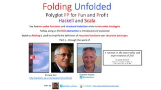
  • 1. See how recursive functions and structural induction relate to recursive datatypes Follow along as the fold abstraction is introduced and explained Watch as folding is used to simplify the definition of recursive functions over recursive datatypes Part 1 - through the work of Folding Unfolded Polyglot FP for Fun and Profit Haskell and Scala Graham Hutton @haskellhutt @philip_schwarzslides by https://www.slideshare.net/pjschwarz Richard Bird http://www.cs.ox.ac.uk/people/richard.bird/
  • 2. Richard Bird @philip_schwarz This slide deck is almost entirely centered on material from Richard Bird’s fantastic book, Introduction to Functional Programming using Haskell. I hope he’ll forgive me for relying so heavily on his work, but I couldn’t resist using extensive excerpts from his compelling book to introduce and explain the concept of folding. http://www.cs.ox.ac.uk/people/richard.bird/ https://en.wikipedia.org/wiki/Richard_Bird_(computer_scientist)
  • 3. 3.1 Natural Numbers The natural numbers are the numbers 0, 1, 2 and so on, used for counting. The type 𝑵𝒂𝒕 is introduced by the declaration 𝐝𝐚𝐭𝐚 𝑵𝒂𝒕 = 𝒁𝒆𝒓𝒐 | 𝑺𝒖𝒄𝒄 𝑵𝒂𝒕 𝑵𝒂𝒕 is our first example of a recursive datatype declaration. The definition says that Zero is a value of 𝑵𝒂𝒕, and that Succ 𝑛 is a value of 𝑵𝒂𝒕 whenever 𝑛 is. In particular, the constructor 𝑺𝒖𝒄𝒄 (short for ‘successor’), has type 𝑵𝒂𝒕 → 𝑵𝒂𝒕. For example, each of 𝒁𝒆𝒓𝒐, 𝑺𝒖𝒄𝒄 𝒁𝒆𝒓𝒐, 𝑺𝒖𝒄𝒄 (𝑺𝒖𝒄𝒄 𝒁𝒆𝒓𝒐) is an element of 𝑵𝒂𝒕. As an element of 𝑵𝒂𝒕 the number 7 would be represented by 𝑺𝒖𝒄𝒄 (𝑺𝒖𝒄𝒄 (𝑺𝒖𝒄𝒄 (𝑺𝒖𝒄𝒄 (𝑺𝒖𝒄𝒄 (𝑺𝒖𝒄𝒄 (𝑺𝒖𝒄𝒄 𝒁𝒆𝒓𝒐)))))) Every natural number is represented by a unique value of 𝑵𝒂𝒕. On the other hand, not every value of 𝑵𝒂𝒕 represents a well- defined natural number. In fact 𝑵𝒂𝒕 also contains the values ⊥, 𝑺𝒖𝒄𝒄 ⊥, 𝑺𝒖𝒄𝒄 (𝑺𝒖𝒄𝒄 ⊥), and so on. These additional values will be discussed later. Let us see how to program the basic arithmetic and comparison operations on 𝑵𝒂𝒕. Addition can be defined by + ∷ 𝑵𝒂𝒕 → 𝑵𝒂𝒕 → 𝑵𝒂𝒕 𝑚 + 𝒁𝒆𝒓𝒐 = 𝑚 𝑚 + 𝑺𝒖𝒄𝒄 𝑛 = 𝑺𝒖𝒄𝒄 𝑚 + 𝑛 This is a recursive definition, defining + by pattern matching on the second argument. Since every element of 𝑵𝒂𝒕, apart for ⊥, is either 𝒁𝒆𝒓𝒐 or of the form Succ 𝑛, where 𝑛 is an element of 𝑵𝒂𝒕, the two patterns in the equations for + are disjoint and cover all numbers apart from ⊥. 
 Richard Bird
  • 4. Here is how 𝒁𝒆𝒓𝒐 + 𝑺𝒖𝒄𝒄 (𝑺𝒖𝒄𝒄 𝒁𝒆𝒓𝒐) would be evaluated: 𝒁𝒆𝒓𝒐 + 𝑺𝒖𝒄𝒄 (𝑺𝒖𝒄𝒄 𝒁𝒆𝒓𝒐) = { second equation for +, i.e. 𝑚 + 𝑺𝒖𝒄𝒄 𝑛 = 𝑺𝒖𝒄𝒄 𝑚 + 𝑛 } 𝑺𝒖𝒄𝒄 𝒁𝒆𝒓𝒐 + 𝑺𝒖𝒄𝒄 𝒁𝒆𝒓𝒐 = { second equation for +, i.e. 𝑚 + 𝑺𝒖𝒄𝒄 𝑛 = 𝑺𝒖𝒄𝒄 𝑚 + 𝑛 } 𝑺𝒖𝒄𝒄 𝑺𝒖𝒄𝒄 (𝒁𝒆𝒓𝒐 + 𝒁𝒆𝒓𝒐) = { first equation for +, i.e. 𝑚 + 𝒁𝒆𝒓𝒐 = 𝑚 } 𝑺𝒖𝒄𝒄 (𝑺𝒖𝒄𝒄 𝒁𝒆𝒓𝒐) 
it is not a practical proposition to introduce natural numbers through the datatype 𝑵𝒂𝒕: arithmetic would be just too inefficient. In particular, calculating 𝑚 + n would require (𝑛 + 1) evaluation steps. On the other hand, counting on your fingers is a good way to understand addition. Given +, we can define ×: (×) ∷ 𝑵𝒂𝒕 → 𝑵𝒂𝒕 → 𝑵𝒂𝒕 𝑚 × 𝒁𝒆𝒓𝒐 = 𝒁𝒆𝒓𝒐 𝑚 × 𝑺𝒖𝒄𝒄 𝑛 = 𝑚 × 𝑛 + 𝑚 Given ×, we can define exponentiation (↑) by (↑) ∷ 𝑵𝒂𝒕 → 𝑵𝒂𝒕 → 𝑵𝒂𝒕 𝑚 ↑ 𝒁𝒆𝒓𝒐 = 𝑺𝒖𝒄𝒄 𝒁𝒆𝒓𝒐 𝑚 ↑ 𝑺𝒖𝒄𝒄 𝑛 = 𝑚 ↑ 𝑛 × 𝑚 
 Richard Bird
  • 5. On the next slide we show the definitions of +, ×, and ↑ again, and have a go at implementing the three operations in Scala, together with some tests.
  • 6. val `(+)`: Nat => Nat => Nat = m => { case Zero => m case Succ(n) => Succ(m + n) } implicit class NatOps(m: Nat){ def +(n: Nat) = `(+)`(m)(n) def ×(n: Nat) = `(×)`(m)(n) def ↑(n: Nat) = `(↑)`(m)(n) } sealed trait Nat case class Succ(n: Nat) extends Nat case object Zero extends Nat + ∷ 𝑵𝒂𝒕 → 𝑵𝒂𝒕 → 𝑵𝒂𝒕 𝑚 + 𝒁𝒆𝒓𝒐 = 𝑚 𝑚 + 𝑺𝒖𝒄𝒄 𝑛 = 𝑺𝒖𝒄𝒄 𝑚 + 𝑛 val `(×)`: Nat => Nat => Nat = m => { case Zero => Zero case Succ(n) => (m × n) + m } val `(↑)`: Nat => Nat => Nat = m => { case Zero => Succ(Zero) case Succ(n) => (m ↑ n) × m } (×) ∷ 𝑵𝒂𝒕 → 𝑵𝒂𝒕 → 𝑵𝒂𝒕 𝑚 × 𝒁𝒆𝒓𝒐 = 𝒁𝒆𝒓𝒐 𝑚 × 𝑺𝒖𝒄𝒄 𝑛 = 𝑚 × 𝑛 + 𝑚 (↑) ∷ 𝑵𝒂𝒕 → 𝑵𝒂𝒕 → 𝑵𝒂𝒕 𝑚 ↑ 𝒁𝒆𝒓𝒐 = 𝑺𝒖𝒄𝒄 𝒁𝒆𝒓𝒐 𝑚 ↑ 𝑺𝒖𝒄𝒄 𝑛 = 𝑚 ↑ 𝑛 × 𝑚 𝐝𝐚𝐭𝐚 𝑵𝒂𝒕 = 𝒁𝒆𝒓𝒐 | 𝑺𝒖𝒄𝒄 𝑵𝒂𝒕 ; assert(0 + 0 == 0) ; assert(Zero + Zero == Zero) ; assert(0 + 1 == 1) ; assert(Zero + Succ(Zero) == Succ(Zero)) ; assert(1 + 0 == 1) ; assert(Succ(Zero) + Zero == Succ(Zero)) ; assert(1 + 1 == 2) ; assert(Succ(Zero) + Succ(Zero) == Succ(Succ(Zero))) ; assert(2 + 3 == 5) ; assert(Succ(Succ(Zero)) + Succ(Succ(Succ(Zero))) == Succ(Succ(Succ(Succ(Succ(Zero)))))) ; assert(0 * 0 == 0) ; assert((Zero × Zero) == Zero) ; assert(1 * 0 == 0) ; assert((Succ(Zero) × Zero) == Zero) ; assert(0 * 1 == 0) ; assert((Zero × Succ(Zero)) == Zero) ; assert(1 * 1 == 1) ; assert((Succ(Zero) × Succ(Zero)) == Succ(Zero)) ; assert(1 * 2 == 2) ; assert((Succ(Zero) × Succ(Succ(Zero))) == Succ(Succ(Zero))) ; assert(2 * 3 == 6) ; assert((Succ(Succ(Zero)) × Succ(Succ(Succ(Zero)))) == Succ(Succ(Succ(Succ(Succ(Succ(Zero))))))) ; assert(Math.pow(1,0) == 1) ; assert( (Succ(Zero) ↑ Zero) == Succ(Zero) ) ; assert(Math.pow(2,2) == 4) ; assert( (Succ(Succ(Zero)) ↑ Succ(Succ(Zero))) == Succ(Succ(Succ(Succ(Zero)))) )
  • 7. The remaining arithmetic operation common to all numbers is subtraction (−). However, subtraction is a partial operation on natural numbers. The definition is − ∷ 𝑵𝒂𝒕 → 𝑵𝒂𝒕 → 𝑵𝒂𝒕 𝑚 − 𝒁𝒆𝒓𝒐 = 𝑚 𝑺𝒖𝒄𝒄 𝑚 − 𝑺𝒖𝒄𝒄 𝑛 = 𝑚 − 𝑛 This definition uses pattern matching on both arguments; taken together, the patterns are disjoint but not exhaustive. For example, 𝑺𝒖𝒄𝒄 𝒁𝒆𝒓𝒐 − 𝑺𝒖𝒄𝒄 (𝑺𝒖𝒄𝒄 𝒁𝒆𝒓𝒐) = { second equation for −, i.e. 𝑺𝒖𝒄𝒄 𝑚 − 𝑺𝒖𝒄𝒄 𝑛 = 𝑚 − 𝑛 } 𝒁𝒆𝒓𝒐 − 𝑺𝒖𝒄𝒄 𝒁𝒆𝒓𝒐 = { case exhaustion } ⊥ The hint ‘case exhaustion’ in the last step indicates that no equation for − has a pattern that matches (𝒁𝒆𝒓𝒐 − 𝑺𝒖𝒄𝒄 𝒁𝒆𝒓𝒐). More generally, 𝑚 − 𝑛 = ⊥ if 𝑚 < 𝑛. The partial nature of subtraction on the natural numbers is the prime motivation for introducing the integer numbers; over the integers, − is a total operation. ...Finally, here are two more examples of programming with 𝑵𝒂𝒕. The factorial and Fibonacci functions are defined by 𝑓𝑎𝑐𝑡 ∷ 𝑵𝒂𝒕 → 𝑵𝒂𝒕 𝑓𝑎𝑐𝑡 𝒁𝒆𝒓𝒐 = 𝑺𝒖𝒄𝒄 𝒁𝒆𝒓𝒐 𝑓𝑎𝑐𝑡 𝑺𝒖𝒄𝒄 𝑛 = 𝑺𝒖𝒄𝒄 𝑛 × 𝑓𝑎𝑐𝑡 𝑛 𝑓𝑖𝑏 ∷ 𝑵𝒂𝒕 → 𝑵𝒂𝒕 𝑓𝑖𝑏 𝒁𝒆𝒓𝒐 = 𝑺𝒖𝒄𝒄 𝒁𝒆𝒓𝒐 𝑓𝑖𝑏 𝑺𝒖𝒄𝒄 𝒁𝒆𝒓𝒐 = 𝑺𝒖𝒄𝒄 𝒁𝒆𝒓𝒐 𝑓𝑖𝑏 𝑺𝒖𝒄𝒄 𝑺𝒖𝒄𝒄 𝑛 = 𝑓𝑖𝑏 𝑺𝒖𝒄𝒄 𝑛 + 𝑓𝑖𝑏 𝑛 Richard Bird
  • 8. See the next slide for a Scala implementation of the − operation.
  • 9. − ∷ 𝑵𝒂𝒕 → 𝑵𝒂𝒕 → 𝑵𝒂𝒕 𝑚 − 𝒁𝒆𝒓𝒐 = 𝑚 𝑺𝒖𝒄𝒄 𝑚 − 𝑺𝒖𝒄𝒄 𝑛 = 𝑚 − 𝑛 val `(-)`: Nat => Nat => Nat = m => n => (m,n) match { case (_,Zero) => m case (Succ(x),Succ(y)) => x - y } ; assert(0 - 0 == 0) ; assert(Zero - Zero == Zero) ; assert(1 - 0 == 1) ; assert(Succ(Zero) - Zero == Succ(Zero)) ; assert(5 - 3 == 2) ; assert(Succ(Succ(Succ(Succ(Succ(Zero))))) - Succ(Succ(Succ(Zero))) == Succ(Succ(Zero))) ; assert(3 - 5 == -2) ; assert( Try { Succ(Succ(Succ(Zero))) - Succ(Succ(Succ(Succ(Succ(Zero))))) }.toString.startsWith( "Failure(scala.MatchError: (Zero,Succ(Succ(Zero)))" ) ) No equation for − has a pattern that matches (𝒁𝒆𝒓𝒐 − 𝑺𝒖𝒄𝒄 𝒁𝒆𝒓𝒐). Similarly for (𝒁𝒆𝒓𝒐 − 𝑺𝒖𝒄𝒄 (𝑺𝒖𝒄𝒄 𝒁𝒆𝒓𝒐)), (𝒁𝒆𝒓𝒐 − 𝑺𝒖𝒄𝒄 (𝑺𝒖𝒄𝒄(𝑺𝒖𝒄𝒄 𝒁𝒆𝒓𝒐))), etc. More generally, 𝑚 − 𝑛 = ⊥ if 𝑚 < 𝑛. 𝑚 − 𝑛 throws scala.MatchError if 𝑚 < 𝑛.
  • 10. @philip_schwarz On the next slide we show the definitions of 𝑓𝑎𝑐𝑡, and 𝑓𝑖𝑏 again, and have a go at implementing the two functions in Scala, together with some tests.
  • 11. val fact: Nat => Nat = { case Zero => Succ(Zero) case Succ(n) => Succ(n) × fact(n) } 𝑓𝑎𝑐𝑡 ∷ 𝑵𝒂𝒕 → 𝑵𝒂𝒕 𝑓𝑎𝑐𝑡 𝒁𝒆𝒓𝒐 = 𝑺𝒖𝒄𝒄 𝒁𝒆𝒓𝒐 𝑓𝑎𝑐𝑡 𝑺𝒖𝒄𝒄 𝑛 = 𝑺𝒖𝒄𝒄 𝑛 × 𝑓𝑎𝑐𝑡 𝑛 𝑓𝑖𝑏 ∷ 𝑵𝒂𝒕 → 𝑵𝒂𝒕 𝑓𝑖𝑏 𝒁𝒆𝒓𝒐 = 𝑺𝒖𝒄𝒄 𝒁𝒆𝒓𝒐 𝑓𝑖𝑏 𝑺𝒖𝒄𝒄 𝒁𝒆𝒓𝒐 = 𝑺𝒖𝒄𝒄 𝒁𝒆𝒓𝒐 𝑓𝑖𝑏 𝑺𝒖𝒄𝒄 𝑺𝒖𝒄𝒄 𝑛 = 𝑓𝑖𝑏 𝑺𝒖𝒄𝒄 𝑛 + 𝑓𝑖𝑏 𝑛 val fib: Nat => Nat = { case Zero => Succ(Zero) case Succ(Zero) => Succ(Zero) case Succ(Succ(n)) => fib(Succ(n)) + fib(n) } def factorial(n: Int): Int = if (n == 0) 1 else n * factorial(n-1) ; assert(factorial(0) == 1) ; assert(fact(Zero) == Succ(Zero)) ; assert(factorial(1) == 1) ; assert(fact(Succ(Zero)) == Succ(Zero)) ; assert(factorial(2) == 2) ; assert(fact(Succ(Succ(Zero))) == Succ(Succ(Zero))) ; assert(factorial(3) == 6) ; assert(fact(Succ(Succ(Succ(Zero)))) == Succ(Succ(Succ(Succ(Succ(Succ(Zero))))))) def fibonacci(n: Int): Int = if (n == 0 || n == 1) 1 else fibonacci(n-1) + fibonacci(n-2) ; assert(fibonacci(0) == 1) ; assert(fib(Zero) == Succ(Zero)) ; assert(fibonacci(1) == 1) ; assert(fib(Succ(Zero)) == Succ(Zero)) ; assert(fibonacci(2) == 2) ; assert(fib(Succ(Succ(Zero))) == Succ(Succ(Zero))) ; assert(fibonacci(3) == 3) ; assert(fib(Succ(Succ(Succ(Zero)))) == Succ(Succ(Succ(Zero)))) ; assert(fibonacci(4) == 5) ; assert(fib(Succ(Succ(Succ(Succ(Zero))))) == Succ(Succ(Succ(Succ(Succ(Zero)))))) ; assert(fibonacci(5) == 8) ; assert(fib(Succ(Succ(Succ(Succ(Succ(Zero)))))) == Succ(Succ(Succ(Succ(Succ(Succ(Succ(Succ(Zero)))))))))
  • 12. 3.1.1 Partial numbers Let us now return to the point about there being extra values in 𝑵𝒂𝒕. The values ⊥, 𝑺𝒖𝒄𝒄 ⊥, 𝑺𝒖𝒄𝒄 (𝑺𝒖𝒄𝒄 ⊥), 
 are all different and each is also a member of 𝑵𝒂𝒕. That they exist is a consequence of three facts: i. ⊥ is an element of 𝑵𝒂𝒕 because every datatype declaration introduces at least one extra value, the undefined value of the type. ii. constructor functions of a datatype are assumed to be nonstrict iii. 𝑺𝒖𝒄𝒄 𝑛 is an element of Nat, whenever 𝑛 is To appreciate why these extra values are different from one another, suppose we define 𝑢𝑛𝑑𝑒𝑓𝑖𝑛𝑒𝑑 ∷ 𝑵𝒂𝒕 by the equation 𝑢𝑛𝑑𝑒𝑓𝑖𝑛𝑒𝑑 = 𝑢𝑛𝑑𝑒𝑓𝑖𝑛𝑒𝑑. Then ? 𝒁𝒆𝒓𝒐 < 𝑢𝑛𝑑𝑒𝑓𝑖𝑛𝑒𝑑 {Interrupted!} ? 𝒁𝒆𝒓𝒐 < 𝑺𝒖𝒄𝒄 𝑢𝑛𝑑𝑒𝑓𝑖𝑛𝑒𝑑 𝑇𝑟𝑢𝑒 ? 𝑺𝒖𝒄𝒄 𝒁𝒆𝒓𝒐 < 𝑺𝒖𝒄𝒄 𝑢𝑛𝑑𝑒𝑓𝑖𝑛𝑒𝑑 {Interrupted!} ? 𝑺𝒖𝒄𝒄 𝒁𝒆𝒓𝒐 < 𝑺𝒖𝒄𝒄 (𝑺𝒖𝒄𝒄 𝑢𝑛𝑑𝑒𝑓𝑖𝑛𝑒𝑑) 𝑇𝑟𝑢𝑒 One can interpret the extra values in the following way: ⊥ corresponds to the natural number about which there is absolutely no information; 𝑺𝒖𝒄𝒄 ⊥ to the natural number about which the only information is that it is greater than 𝒁𝒆𝒓𝒐; 𝑺𝒖𝒄𝒄 (𝑺𝒖𝒄𝒄 ⊥) to the natural number about which the only information is that it is greater than 𝑺𝒖𝒄𝒄 𝒁𝒆𝒓𝒐; and so on. Richard Bird
  • 13. There is also one further value of 𝑵𝒂𝒕, namely the ‘infinite’ number: 𝑺𝒖𝒄𝒄 (𝑺𝒖𝒄𝒄 (𝑺𝒖𝒄𝒄 (𝑺𝒖𝒄𝒄 
 ))) This number can be defined by 𝑖𝑛𝑓𝑖𝑛𝑖𝑡𝑊 ∷ 𝑵𝒂𝒕 𝑖𝑛𝑓𝑖𝑛𝑖𝑡𝑊 = 𝑺𝒖𝒄𝒄 𝑖𝑛𝑓𝑖𝑛𝑖𝑡𝑊 It is different from all the other numbers, because it is the only number 𝑥 for which 𝑺𝒖𝒄𝒄 𝑚 < 𝑥 returns 𝑻𝒓𝒖𝒆 for all finite numbers 𝑚. In this sense, 𝑖𝑛𝑓𝑖𝑛𝑖𝑡𝑊 is the largest element of 𝑵𝒂𝒕. If we request the value of 𝑖𝑛𝑓𝑖𝑛𝑖𝑡𝑊, then we obtain ? 𝑖𝑛𝑓𝑖𝑛𝑖𝑡𝑊 𝑺𝒖𝒄𝒄 (𝑺𝒖𝒄𝒄 (𝑺𝒖𝒄𝒄 (𝑺𝒖𝒄𝒄 (𝑺𝒖𝒄𝒄 {𝐌𝑛𝑡𝑒𝑟𝑟𝑢𝑝𝑡𝑒𝑑!} The number 𝑖𝑛𝑓𝑖𝑛𝑖𝑡𝑊 satisfies other properties, in particular 𝑛 + 𝑖𝑛𝑓𝑖𝑛𝑖𝑡𝑊 = 𝑖𝑛𝑓𝑖𝑛𝑖𝑡𝑊, for all numbers 𝑛. The dual equation 𝑖𝑛𝑓𝑖𝑛𝑖𝑡𝑊 + 𝑛 = 𝑖𝑛𝑓𝑖𝑛𝑖𝑡𝑊 holds only for finite numbers 𝑛. We will see how to prove assertions such as these in the next section. To summarise this discussion, we can divide the values of 𝑵𝒂𝒕 into three classes: • The finite numbers, those that correspond to well-defined natural numbers. • The partial numbers, ⊥, 𝑺𝒖𝒄𝒄 ⊥, and so on. • The infinite numbers, of which there is just one, namely 𝑖𝑛𝑓𝑖𝑛𝑖𝑡𝑊. We will see that this classification holds true of all recursive types. There will be the finite elements of the type, the partial elements, and the infinite elements. Although the infinite natural number is not of much use, the same is not true of the infinite values of other datatypes. 
 Richard Bird
  • 14. Note that when in this slide deck we mention the concepts of ⊥ and 𝑖𝑛𝑓𝑖𝑛𝑖𝑡𝑊, it is mainly in a Haskell context, as we did in the last two slides. In particular, we won’t be modelling ⊥ and 𝑖𝑛𝑓𝑖𝑛𝑖𝑡𝑊 in any of the Scala code you’ll see throughout the deck.
  • 15. 3.2 Induction In order to reason about the properties of recursively defined functions over a recursive datatype, we can appeal to a principle of structural induction. In the case of 𝑵𝒂𝒕, the principle of structural induction can be defined as follows: In order to show that some property 𝑃(𝑛) holds for each finite number 𝑛 of 𝑵𝒂𝒕, it is sufficient to show: Case (𝒁𝒆𝒓𝒐). That 𝑃(𝒁𝒆𝒓𝒐) holds. Case (𝑺𝒖𝒄𝒄 𝑛). That if 𝑃(𝑛) holds, then 𝑃(𝑺𝒖𝒄𝒄 𝑛) holds also. Induction is valid for the same reason that recursive definitions are valid: every finite number is either 𝒁𝒆𝒓𝒐 or of the form 𝑺𝒖𝒄𝒄 𝑛, where 𝑛 is a finite number. If we prove the first case, then we have shown that the property is true for 𝒁𝒆𝒓𝒐; If we also prove the second case, then we have shown that the property is true for 𝑺𝒖𝒄𝒄 𝒁𝒆𝒓𝒐, since it is true for 𝒁𝒆𝒓𝒐. But now, by the same argument, it is true for 𝑺𝒖𝒄𝒄 𝑺𝒖𝒄𝒄 𝒁𝒆𝒓𝒐 , and so on. The principle needs to be extended if we want to assert that some proposition is true for all elements of 𝑵𝒂𝒕, but we postpone discussion of this point for the following section. As an example, let’s prove that 𝒁𝒆𝒓𝒐 + 𝑛 = 𝑛 for all finite numbers 𝑛. Recall that + is defined by 𝑚 + 𝒁𝒆𝒓𝒐 = 𝑚 𝑚 + 𝑺𝒖𝒄𝒄 𝑛 = 𝑺𝒖𝒄𝒄 𝑚 + 𝑛 The first equation asserts that 𝒁𝒆𝒓𝒐 is a right unit of +. In general, 𝑒 is a left unit of ⊕ if 𝑒 ⊕ 𝑥 = 𝑥 for all 𝑥, and a right unit of 𝑥 if 𝑥 ⊕ 𝑒 = 𝑥 for all 𝑥. If 𝑒 is both a left unit and a right unit of an operator ⊕, then it is called the unit of ⊕. The terminology is appropriate since only one value can be both a left and right unit. So, by proving that 𝒁𝒆𝒓𝒐 is a left unit , we have proved that 𝒁𝒆𝒓𝒐 is the unit of +. Richard Bird
  • 16. Proof. The proof is by induction on 𝑛. More precisely, we take for 𝑃(𝑛) the assertion that 𝒁𝒆𝒓𝒐 + 𝑛 = 𝑛. This equation is referred to as the induction hypothesis. Case (𝒁𝒆𝒓𝒐). We have to show 𝒁𝒆𝒓𝒐 + 𝒁𝒆𝒓𝒐 = 𝒁𝒆𝒓𝒐, which is immediate from the first equation defining +. Case (𝑺𝒖𝒄𝒄 𝑛). We have to show that 𝒁𝒆𝒓𝒐 + 𝑺𝒖𝒄𝒄 𝑛 = 𝑺𝒖𝒄𝒄 𝑛, which we do by simplifying the left-hand expression: 𝒁𝒆𝒓𝒐 + 𝑺𝒖𝒄𝒄 𝑛 = { second equation for +, i.e. 𝑚 + 𝑺𝒖𝒄𝒄 𝑛 = 𝑺𝒖𝒄𝒄 𝑚 + 𝑛 } 𝑺𝒖𝒄𝒄 (𝒁𝒆𝒓𝒐 + 𝑛) = { induction hypothesis} 𝑺𝒖𝒄𝒄 𝑛 ☐ This example shows the format we will use for inductive proofs, laying out each case separately and using a ☐ to mark the end. The very last step made use of the induction hypothesis, which is allowed by the way induction works. 
 3.2.1 Full Induction In the form given above, the induction principle for 𝑵𝒂𝒕 suffices only to prove properties of the finite members of 𝑵𝒂𝒕. If we want to show that a property 𝑃 also hold for every partial number, then we have to prove three things: Case (⊥). That 𝑃(⊥) holds. Case (𝒁𝒆𝒓𝒐). That 𝑃(𝒁𝒆𝒓𝒐) holds. Case (𝑺𝒖𝒄𝒄 𝑛). That if 𝑃(𝑛) holds, then 𝑃(𝑺𝒖𝒄𝒄 𝑛) holds also. We can omit the second case, but then we can conclude only that 𝑃(𝑛) holds for every partial number. The reason the principle is valid is that is that every partial number is either ⊥ or of the form 𝑺𝒖𝒄𝒄 𝑛 for some partial number 𝑛. Richard Bird
  • 17. To illustrate, let us prove the somewhat counterintuitive result that 𝑚 + 𝑛 = 𝑛 for all numbers 𝑚 and all partial numbers 𝑛. Proof. The proof is by partial number induction on 𝑛. Case (⊥). The equation 𝑚 + ⊥ = ⊥ follows at once by case exhaustion in the definition of +. That is, ⊥ does not match either of the patterns 𝒁𝒆𝒓𝒐 or 𝑺𝒖𝒄𝒄 𝑛. Case (𝑺𝒖𝒄𝒄 𝑛). For the left-hand side, we reason 𝑚 + 𝑺𝒖𝒄𝒄 𝑛 = { second equation for +, i.e. 𝑚 + 𝑺𝒖𝒄𝒄 𝑛 = 𝑺𝒖𝒄𝒄 𝑚 + 𝑛 } 𝑺𝒖𝒄𝒄 (𝑚 + 𝑛) = { induction hypothesis} 𝑺𝒖𝒄𝒄 𝑛 Since the right-hand side is also 𝑺𝒖𝒄𝒄 𝑛, we are done. 3.2.2 Program synthesis In the proofs above we defined some functions and then used induction to prove a certain property. We can also view induction as a way to synthesise definitions of functions so that they satisfy the properties we want. Let us illustrate with a simple example. Suppose we specify subtraction of natural numbers by the condition 𝑚 + 𝑛 − 𝑛 = 𝑚 for all 𝑚 and 𝑛. The specification does not give a constructive definition of − , merely a property that it has to satisfy. However, we can do an induction proof on 𝑛 of the equation above, but view the calculation as a way of generating a suitable definition of − . Richard Bird
  • 18. Unlike previous proofs, we reason with the equation as a whole, since simplification of both sides independently is not possible if we do not know what all the rules of simplification are. Case (𝒁𝒆𝒓𝒐). We reason 𝑚 + 𝒁𝒆𝒓𝒐 − 𝒁𝒆𝒓𝒐 = 𝑚 ≡ { first equation for +, i.e. 𝑚 + 𝒁𝒆𝒓𝒐 = 𝑚 } 𝑚 − 𝒁𝒆𝒓𝒐 = 𝑚 Hence we can take 𝑚 − 𝒁𝒆𝒓𝒐 = 𝑚 to satisfy the case. The symbol ≡ is used to separate steps of the calculation since we are calculating with mathematical assertions, not with values of a datatype. Case (𝑺𝒖𝒄𝒄 𝑛). We reason 𝑚 + 𝑺𝒖𝒄𝒄 𝑛 − 𝑺𝒖𝒄𝒄 𝑛 = 𝑚 ≡ { second equation for +, i.e. 𝑚 + 𝑺𝒖𝒄𝒄 𝑛 = 𝑺𝒖𝒄𝒄 𝑚 + 𝑛 } 𝑺𝒖𝒄𝒄 𝑚 + 𝑛 − 𝑺𝒖𝒄𝒄 𝑛 = 𝑚 ≡ { hypothesis 𝑚 + 𝑛 − 𝑛 = 𝑚} 𝑺𝒖𝒄𝒄 𝑚 + 𝑛 − 𝑺𝒖𝒄𝒄 𝑛 = 𝑚 + 𝑛 − 𝑛 Replacing 𝑚 + 𝑛 in the last equation by 𝑚, we can take 𝑺𝒖𝒄𝒄 𝑚 − 𝑺𝒖𝒄𝒄 𝑛 = 𝑚 − 𝑛 to satisfy the case. Hence we have derived 𝑚 − 𝒁𝒆𝒓𝒐 = 𝑚 𝑺𝒖𝒄𝒄 𝑚 − 𝑺𝒖𝒄𝒄 𝑛 = 𝑚 − 𝑛 This is the program for − seen earlier. Richard Bird
  • 19. After that look at structural induction, it is finally time to see how Richard Bird introduces the concept of folding.
  • 20. 3.3 The fold function Many of the recursive definitions seen so far have a common pattern, exemplified by the following definition of a function 𝑓: 𝑓 ∷ 𝑵𝒂𝒕 → 𝐎 𝑓 𝒁𝒆𝒓𝒐 = 𝑐 𝑓 𝑺𝒖𝒄𝒄 𝑛 = ℎ 𝑓 𝑛 Here, 𝐎 is some type, 𝑐 is an element of 𝐎, and ℎ ∷ 𝐎 → 𝐎 . Observe that 𝑓 works by taking an element of 𝑵𝒂𝒕 and replacing 𝒁𝒆𝒓𝒐 by 𝑐 and 𝑺𝒖𝒄𝒄 by ℎ. For example, 𝑓 takes 𝑺𝒖𝒄𝒄 (𝑺𝒖𝒄𝒄 (𝑺𝒖𝒄𝒄 𝒁𝒆𝒓𝒐)) to ℎ (ℎ (ℎ 𝑐)) The two equations for 𝑓 can be captured in terms of a single function, 𝑓𝑜𝑙𝑑𝑛, called the 𝑓𝑜𝑙𝑑 function for 𝑵𝒂𝒕. The definition is 𝑓𝑜𝑙𝑑𝑛 ∷ 𝛌 → 𝛌 → 𝛌 → 𝑵𝒂𝒕 → 𝛌 𝑓𝑜𝑙𝑑𝑛 ℎ 𝑐 𝒁𝒆𝒓𝒐 = 𝑐 𝑓𝑜𝑙𝑑𝑛 ℎ 𝑐 𝑺𝒖𝒄𝒄 𝑛 = ℎ 𝑓𝑜𝑙𝑑𝑛 ℎ 𝑐 𝑛 In particular, we have 𝑚 + 𝑛 = 𝑓𝑜𝑙𝑑𝑛 𝑺𝒖𝒄𝒄 𝑚 𝑛 𝑚 × 𝑛 = 𝑓𝑜𝑙𝑑𝑛 + 𝑚 𝒁𝒆𝒓𝒐 𝑛 𝑚 ↑ 𝑛 = 𝑓𝑜𝑙𝑑𝑛 × 𝑚 𝑺𝒖𝒄𝒄 𝒁𝒆𝒓𝒐 𝑛 It follows also that the identity function 𝑖𝑑 on 𝑵𝒂𝒕 satisfies 𝑖𝑑 = 𝑓𝑜𝑙𝑑𝑛 𝑺𝒖𝒄𝒄 𝒁𝒆𝒓𝒐. A suitable 𝑓𝑜𝑙𝑑 function can be defined for every recursive type, and we will see other 𝑓𝑜𝑙𝑑 functions in the following chapters. Richard Bird
  • 21. + ∷ 𝑵𝒂𝒕 → 𝑵𝒂𝒕 → 𝑵𝒂𝒕 𝑚 + 𝒁𝒆𝒓𝒐 = 𝑚 𝑚 + 𝑺𝒖𝒄𝒄 𝑛 = 𝑺𝒖𝒄𝒄 𝑚 + 𝑛 (×) ∷ 𝑵𝒂𝒕 → 𝑵𝒂𝒕 → 𝑵𝒂𝒕 𝑚 × 𝒁𝒆𝒓𝒐 = 𝒁𝒆𝒓𝒐 𝑚 × 𝑺𝒖𝒄𝒄 𝑛 = 𝑚 × 𝑛 + 𝑚 (↑) ∷ 𝑵𝒂𝒕 → 𝑵𝒂𝒕 → 𝑵𝒂𝒕 𝑚 ↑ 𝒁𝒆𝒓𝒐 = 𝑺𝒖𝒄𝒄 𝒁𝒆𝒓𝒐 𝑚 ↑ 𝑺𝒖𝒄𝒄 𝑛 = 𝑚 ↑ 𝑛 × 𝑚 + ∷ 𝑵𝒂𝒕 → 𝑵𝒂𝒕 → 𝑵𝒂𝒕 𝑚 + 𝑛 = 𝑓𝑜𝑙𝑑𝑛 𝑺𝒖𝒄𝒄 𝑚 𝑛 (×) ∷ 𝑵𝒂𝒕 → 𝑵𝒂𝒕 → 𝑵𝒂𝒕 𝑚 × 𝑛 = 𝑓𝑜𝑙𝑑𝑛 + 𝑚 𝒁𝒆𝒓𝒐 𝑛 (↑) ∷ 𝑵𝒂𝒕 → 𝑵𝒂𝒕 → 𝑵𝒂𝒕 𝑚 ↑ 𝑛 = 𝑓𝑜𝑙𝑑𝑛 × 𝑚 𝑺𝒖𝒄𝒄 𝒁𝒆𝒓𝒐 𝑛 𝑓𝑜𝑙𝑑𝑛 ∷ 𝛌 → 𝛌 → 𝛌 → 𝑵𝒂𝒕 → 𝛌 𝑓𝑜𝑙𝑑𝑛 ℎ 𝑐 𝒁𝒆𝒓𝒐 = 𝑐 𝑓𝑜𝑙𝑑𝑛 ℎ 𝑐 𝑺𝒖𝒄𝒄 𝑛 = ℎ 𝑓𝑜𝑙𝑑𝑛 ℎ 𝑐 𝑛 @philip_schwarz Just to reinforce the ideas on the previous slide, here are the original definitions of +, × and ↑, and next to them, the new definitions in terms of 𝑓𝑜𝑙𝑑𝑛. And the next slide is the same but in terms of Scala code.
  • 22. val `(+)`: Nat => Nat => Nat = m => { case Zero => m case Succ(n) => Succ(m + n) } val `(×)`: Nat => Nat => Nat = m => { case Zero => Zero case Succ(n) => (m × n) + m } val `(↑)`: Nat => Nat => Nat = m => { case Zero => Succ(Zero) case Succ(n) => (m ↑ n) × m } val `(×)`: Nat => Nat => Nat = m => n => foldn((x:Nat) => x + m, Zero, n) def foldn[A](h: A => A, c: A, n: Nat): A = n match { case Zero => c case Succ(n) => h(foldn(h,c,n)) } val `(↑)`: Nat => Nat => Nat = m => n => foldn((x:Nat) => x × m, Succ(Zero), n) val `(+)`: Nat => Nat => Nat = m => n => foldn(Succ,m,n)
  • 23. In the examples above, each instance of 𝑓𝑜𝑙𝑑𝑛 also returned an element of 𝑵𝒂𝒕. In the following two examples, 𝑓𝑜𝑙𝑑𝑛 returns an element of (𝑵𝒂𝒕, 𝑵𝒂𝒕): 𝑓𝑎𝑐𝑡 ∷ 𝑵𝒂𝒕 → 𝑵𝒂𝒕 𝑓𝑎𝑐𝑡 = 𝑠𝑛𝑑 Å  𝑓𝑜𝑙𝑑𝑛 𝑓 (𝒁𝒆𝒓𝒐, 𝑺𝒖𝒄𝒄 𝒁𝒆𝒓𝒐) where 𝑓 𝑚, 𝑛 = (𝑺𝒖𝒄𝒄 𝑚, 𝑺𝒖𝒄𝒄 (𝑚) × 𝑛) 𝑓𝑖𝑏 ∷ 𝑵𝒂𝒕 → 𝑵𝒂𝒕 𝑓𝑖𝑏 = 𝑓𝑠𝑡 Å  𝑓𝑜𝑙𝑑𝑛 𝑔 (𝒁𝒆𝒓𝒐, 𝑺𝒖𝒄𝒄 𝒁𝒆𝒓𝒐) where 𝑔 𝑚, 𝑛 = (𝑛, 𝑚 + 𝑛) The function 𝑓𝑎𝑐𝑡 computes the factorial function and function 𝑓𝑖𝑏 computes the Fibonacci function. Each program works by first computing a more general result, namely an element of (𝑵𝒂𝒕, 𝑵𝒂𝒕), and then extracts the required result. In fact, 𝑓𝑜𝑙𝑑𝑛 𝑓 𝒁𝒆𝒓𝒐, 𝑺𝒖𝒄𝒄 𝒁𝒆𝒓𝒐 𝑛 = 𝑛, 𝑓𝑎𝑐𝑡 𝑛 𝑓𝑜𝑙𝑑𝑛 𝑔 𝒁𝒆𝒓𝒐, 𝑺𝒖𝒄𝒄 𝒁𝒆𝒓𝒐 𝑛 = 𝑓𝑖𝑏 𝑛, 𝑓𝑖𝑏 𝑺𝒖𝒄𝒄 𝑛 These equations can be proved by induction. The program for 𝑓𝑖𝑏 is more efficient than a direct recursive definition. The recursive program requires an exponential number of + operations, while the program above requires only a linear number. We will discuss efficiency in more detail in chapter 7, where the programming technique that led to the invention of the new program for 𝑓𝑖𝑏 will be studied in a more general setting. There are two advantages of writing recursive definitions in terms of 𝑓𝑜𝑙𝑑𝑛. Firstly, the definition is shorter; rather than having to write down two equations, we have only to write down one. Secondly, it is possible to prove general properties of 𝑓𝑜𝑙𝑑𝑛 and use them to prove properties of specific instantiations. In other words, rather than having to write down many induction proofs, we have only to write down one. Richard Bird
  • 24. Now let’s have a very quick look at the datatype for lists, and at induction over lists.
  • 25. 4.1.1 Lists as a datatype A list can be constructed from scratch by starting with the empty list and successively adding elements one by one. One can add elements to the front of the list, or to the rear, or to somewhere in the middle. In the following datatype declaration, nonempty lists are constructed by adding elements to the front of the list: 𝐝𝐚𝐭𝐚 𝑳𝒊𝒔𝒕 𝛌 = 𝑵𝒊𝒍 | 𝑪𝒐𝒏𝒔 𝛌 (𝑳𝒊𝒔𝒕 𝛌) 
The constructor (short for ‘construct’ – the name goes back to the programming language LISP) adds an element to the front of the list. For example, the list 1,2,3 would be represented as the following element of 𝑳𝒊𝒔𝒕 𝑰𝒏𝒕: 𝑪𝒐𝒏𝒔 1 (𝑪𝒐𝒏𝒔 2 (𝑪𝒐𝒏𝒔 3 𝑵𝒊𝒍 )) In functional programming, lists are defined as elements of 𝑳𝒊𝒔𝒕 𝛌. The syntax [𝛌] is used instead of 𝑳𝒊𝒔𝒕 𝛌, the constructor 𝑵𝒊𝒍 is written as [ ], and the constructor 𝑪𝒐𝒏𝒔 is written as infix operator (∶). Moreover, (∶) associates to the right, so 1,2,3 = 1: 2: 3: [ ] = 1 ∶ 2 ∶ 3 ∶ [ ] In other words, the special syntax on the left can be regarded as an abbreviation for the syntax on the right, which is also special, but only by virtue of the fact that the constructors are given nonstandard names. Like functions over other datatypes, functions over lists can be defined by pattern matching. Richard Bird
  • 26. Before moving on to the topic of induction over lists, Richard Bird gives an example of a function defined over lists using pattern matching, but the function he chooses is the equality function, whereas we are going to choose the sum function, just to keep things simpler. 𝑠𝑢𝑚 ∷ [𝑰𝒏𝒕] → 𝑰𝒏𝒕 𝑠𝑢𝑚 [ ] = 0 𝑠𝑢𝑚 𝑥: 𝑥𝑠 = 𝑥 + (𝑠𝑢𝑚 𝑥𝑠) val sum : List[Int] => Int = { case Nil => 0 case x :: xs => x + sum(xs) } assert( sum( 4 :: (5 :: (6 :: Nil)) ) == 15)
  • 27. sealed trait Nat case class Succ(n: Nat) extends Nat case object Zero extends Nat sealed trait List[+A] case class Cons[+A](head: A, tail: List[A]) extends List[A] case object Nil extends List[Nothing] val `(+)`: Nat => Nat => Nat = m => { case Zero => m case Succ(n) => Succ(m + n) } implicit class NatSyntax(m: Nat){ def +(n: Nat) = `(+)`(m)(n) } val sum: List[Nat] => Nat = { case Nil => Zero case Cons(x, xs) => x + sum(xs) } assert( sum( Cons( Succ(Zero), // 1 Cons( Succ(Succ(Zero)), // 2 Cons( Succ(Succ(Succ(Zero))), // 3 Nil))) ) == Succ(Succ(Succ(Succ(Succ(Succ(Zero))))))) // 6 𝑠𝑢𝑚 ∷ 𝑳𝒊𝒔𝒕 𝑵𝒂𝒕 → 𝑵𝒂𝒕 𝑠𝑢𝑚 𝑵𝒊𝒍 = 𝒁𝒆𝒓𝒐 𝑠𝑢𝑚 𝑪𝒐𝒏𝒔 𝑥 𝑥𝑠 = 𝑥 + (𝑠𝑢𝑚 𝑥𝑠) + ∷ 𝑵𝒂𝒕 → 𝑵𝒂𝒕 → 𝑵𝒂𝒕 𝑚 + 𝒁𝒆𝒓𝒐 = 𝑚 𝑚 + 𝑺𝒖𝒄𝒄 𝑛 = 𝑺𝒖𝒄𝒄 𝑚 + 𝑛 𝐝𝐚𝐭𝐚 𝑵𝒂𝒕 = 𝒁𝒆𝒓𝒐 | 𝑺𝒖𝒄𝒄 𝑵𝒂𝒕 𝐝𝐚𝐭𝐚 𝐋𝐢𝐬𝐭 α = 𝐍𝐢𝐥 | 𝐂𝐚𝐧𝐬 α (𝐋𝐢𝐬𝐭 α) Same as on the previous slide, but this time using Nat rather than Int, just for fun.
  • 28. 4.1.2 Induction over Lists Recall from section 3.2 that, for the datatype 𝑵𝒂𝒕 of natural numbers, structural induction is based on three cases: every element of 𝑵𝒂𝒕 is either ⊥, or 𝒁𝒆𝒓𝒐, or else has the form 𝑺𝒖𝒄𝒄 𝑛 for some element 𝑛 of 𝑵𝒂𝒕. Similarly, structural induction on lists is also based on on three cases: every list is either the undefined list ⊥, the empty list [ ], or else has the form 𝑥: 𝑥𝑠 for some 𝑥 and list 𝑥𝑠. To show by induction that a proposition 𝑃(𝑥𝑠) holds for all lists 𝑥𝑠 it suffices therefore to establish three cases: Case (⊥). That 𝑃(⊥) holds. Case ([ ]). That 𝑃([ ]) holds. Case 𝑥: 𝑥𝑠 . That if 𝑃(𝑥𝑠) holds, then 𝑃(𝑥: 𝑥𝑠) also holds for every 𝑥. If we prove only the second two cases, then we can conclude only that 𝑃(𝑥𝑠) holds for every finite list; if we prove only the first and third cases. Then we can conclude only that 𝑃(𝑥𝑠) holds for every partial list. If 𝑃 takes the form of an equation, as all of our laws do, then proving the first and third cases is sufficient to show that 𝑃(𝑥𝑠) holds for every infinite list. Partial lists and infinite lists are described in the following section. Examples of induction proofs are given throughout the remainder of the chapter. Richard Bird
  • 29. Richard Bird provides other examples of recursive functions over lists. Let’s see some of them: list concatenation, flattening of lists of lists, list reversal and length of a list. When looking at the first one, i.e. concatenation, let’s also see an example of proof by structural induction on lists. @philip_schwarz
  • 30. 4.2.1 Concatenation Two lists can be concatenated to form one longer list. This function is denoted by the binary operator ⧺ (pronounced ‘concatenate’). As two simple examples, we have ? 1,2,3 ⧺ 4,5 1,2,3,4,5 ? 1,2 ⧺ ⧺ 1 1,2,1 The formal definition of ⧺ is (⧺) ∷ [α] → [α] → [α] ⧺ 𝑊𝑠 = 𝑊𝑠 𝑥: 𝑥𝑠 ⧺ 𝑊𝑠 = 𝑥 ∶ (𝑥𝑠 ⧺ 𝑊𝑠) Concatenation takes two lists, both of the same type, and produces a third list, again of the same type. Hence the type assignment. The definition of ⧺ is by pattern matching on the left-hand argument; the two patterns are disjoint and cover all cases, apart from the undefined list ⊥. It follows by case exhaustion that ⊥ ⧺ 𝑊𝑠 = ⊥. However, it is not the case that 𝑊𝑠 ⧺ ⊥ = ⊥. For example, ? 1,2,3 ⧺ 𝑢𝑛𝑑𝑒𝑓𝑖𝑛𝑒𝑑 1,2,3{𝐌𝑛𝑡𝑒𝑟𝑟𝑢𝑝𝑡𝑒𝑑!} The list 1,2,3 ⧺ ⊥ is a partial list; In full form it is the list 1: 2: 3: ⊥. The evaluator can compute the first three elements, but thereafter it goes into a nonterminating computation, so we interrupt it. The second equation for ⧺ is very succinct and requires some thought. Once one has come to grips with the definition of ⧺, one Richard Bird
  • 31. has understood a good deal about how lists work in functional programming. Note that the number of steps required to compute 𝑥𝑠 ⧺ 𝑊𝑠 is proportional to the number of elements in 𝑥𝑠. 1, 2 ⧺ 3, 4, 5 = { notation} (1 ∶ 2 ∶ ⧺ (3 ∶ (4 ∶ 5 ∶ [ ] )) = { second equation for ⧺, i.e. 𝑥: 𝑥𝑠 ⧺ 𝑊𝑠 = 𝑥 ∶ (𝑥𝑠 ⧺ 𝑊𝑠) } 1 ∶ ( 2 ∶ ⧺ (3 ∶ (4 ∶ 5 ∶ [ ] ))) = { second equation for ⧺ } 1 ∶ (2 ∶ ( ⧺ (3 ∶ (4 ∶ 5 ∶ [ ] )))) = { first equation for ⧺ i.e. , ⧺ 𝑊𝑠 = 𝑊𝑠 } 1 ∶ (2 ∶ (3 ∶ (4 ∶ 5 ∶ [ ] ))) = { notation} 1, 2, 3, 4, 5 Concatenation is an associative operation with with unit : 𝑥𝑠 ⧺ 𝑊𝑠 ⧺ 𝑧𝑠 = 𝑥𝑠 ⧺ (𝑊𝑠 ⧺ 𝑧𝑠) 𝑥𝑠 ⧺ = ⧺ 𝑥𝑠 = 𝑥𝑠 Let us now prove by induction that ⧺ is associative. Proof. The proof is by induction on 𝑥𝑠. Case (⊥). For the left-hand side, we reason ⊥ ⧺ (𝑊𝑠 ⧺ 𝑧𝑠) = { case exhaustion} ⊥ ⧺ 𝑧𝑠 = { case exhaustion} ⊥ Richard Bird
  • 32. The right-hand side simplifies to ⊥ as well, establishing the case. Case ([ ]). For the left hand side, we reason [ ] ⧺ (𝑊𝑠 ⧺ 𝑧𝑠) = { first equation for ⧺ i.e. , ⧺ 𝑊𝑠 = 𝑊𝑠 } (𝑊𝑠 ⧺ 𝑧𝑠) The right-hand side simplifies to(𝑊𝑠 ⧺ 𝑧𝑠) as well, establishing the case. Case 𝑥 ∶ 𝑥𝑠 . For the left hand side, we reason ((x ∶ 𝑥𝑠) ⧺ 𝑊𝑠) ⧺ 𝑧𝑠 = { second equation for ⧺, i.e. 𝑥: 𝑥𝑠 ⧺ 𝑊𝑠 = 𝑥 ∶ (𝑥𝑠 ⧺ 𝑊𝑠) } ( 𝑥 ∶ 𝑥𝑠 ⧺ 𝑊𝑠) ⧺ 𝑧𝑠 = { second equation for ⧺ } 𝑥 ∶ ( 𝑥𝑠 ⧺ 𝑊𝑠 ⧺ 𝑧𝑠) = { induction hypothesis } 𝑥 ∶ (𝑥𝑠 ⧺ 𝑊𝑠 ⧺ 𝑧𝑠) For the right-hand side we reason (x ∶ 𝑥𝑠) ⧺ (𝑊𝑠 ⧺ 𝑧𝑠) = { second equation for ⧺, i.e. 𝑥 ∶ 𝑥𝑠 ⧺ 𝑊𝑠 = 𝑥 ∶ (𝑥𝑠 ⧺ 𝑊𝑠) } 𝑥 ∶ (𝑥𝑠 ⧺ (𝑊𝑠 ⧺ 𝑧𝑠)) The two sides are equal, establishing the case. 
Note that associativity is proved for all lists, finite, partial or infinite. Hence we can assert that ⧺ is associative without qualification
. Richard Bird
  • 33. 4.2.2 Concat Concatenation performs much the same function for lists as the union operator ∪ does for sets. A companion function is concat, which concatenates a list of lists into one long list. This function, which roughly corresponds to the big-union operator ⋃ for sets of sets, is defined by concat ∷ [ α ] → [α] concat = concat 𝑥𝑠: 𝑥𝑠𝑠 = 𝑥𝑠 ⧺ 𝑐𝑜𝑛𝑐𝑎𝑡 𝑥𝑠𝑠 For example, ?[ 1, 2 ⧺ ⧺ 3, 2,1 ] 1,2,3, 2,1 4.2.3 Reverse Another basic function on lists is reverse, the function that reverses the order of elements in a finite list. For example: ? reverse “Madam, I’m Adam.” “.MadA m’I ,madaM” The definition is reverse ∷ α → [α] reverse = reverse 𝑥 ∶ 𝑥𝑠 = 𝑟𝑒𝑣𝑒𝑟𝑠𝑒 𝑥𝑠 ⧺ [𝑥] In words, to reverse a list 𝑥 ∶ 𝑥𝑠 , one reverses 𝑥𝑠, and then adds 𝑥 to the end. As a program, the above definition is not very Richard Bird
  • 34. efficient: on a list of length 𝑛, it will need a number of reduction steps proportional to 𝑛2 to deliver the reversed list. The first element will be appended to the end of a list of length 𝑛 − 1 , which will take about 𝑛 − 1 steps, the second element will be appended to a list of length 𝑛 − 2 , taking 𝑛 − 2 steps, and so on. The total time is therefore about 𝑛 − 1 + 𝑛 − 2 + ⋯ 1 = 𝑛(𝑛 − 1)/2 steps A more precise analysis is given in chapter 7, and a more efficient program for reverse is given in section 4.5. 4.2.2 Length The length of a list is the number of elements it contains: 𝑙𝑒𝑛𝑔𝑡ℎ ∷ [α] → 𝑰𝒏𝒕 𝑙𝑒𝑛𝑔𝑡ℎ [ ] = 0 𝑙𝑒𝑛𝑔𝑡ℎ 𝑥: 𝑥𝑠 = 1 + 𝑙𝑒𝑛𝑔𝑡ℎ 𝑥𝑠 The nature of the list element is irrelevant when computing the length of a list, whence the type assignment. For example, ? 𝑙𝑒𝑛𝑔𝑡ℎ [𝑢𝑛𝑑𝑒𝑓𝑖𝑛𝑒𝑑, 𝑢𝑛𝑑𝑒𝑓𝑖𝑛𝑒𝑑] 2 However, not every list has a well-defined length. In particular, the partial lists ⊥, 𝑥 ∶ ⊥, 𝑥 ∶ 𝑊 ∶ ⊥, and so on, have an undefined length. Only finite lists have well-defined lengths. The list ⊥, ⊥ is a finite list, not a partial list, because it is the list ⊥ ∶ ⊥ ∶ [ ], which ends in [ ], not ⊥. The computer cannot produce the elements, but it can produce the length of the list. 
 Richard Bird
  • 35. 4.3 Map and filter Two useful functions on lists are map and £ilter. The function map applies a function to each element of a list. For example ? 𝑚ap square [9, 3] ? 𝑚ap (<3) [1, 2, 3] ? 𝑚ap nextLetter “HAL” [81, 9] [𝑇𝑟𝑢𝑒, 𝑇𝑟𝑢𝑒, 𝐹𝑎𝑙𝑠𝑒] “IBM” The definition is map ∷ (α → 𝛜) → [α] → [𝛜] map f = map f 𝑥 ∶ 𝑥𝑠 = 𝑓 𝑥 ∶ map 𝑓 𝑥𝑠 
 4.3 filter The second function, filter, takes a Boolean function p and a list xs and returns that sublist of xs whose elements satisfy p. For example, ? £ilter even [1,2,4,5,32] ? (sum Å  map square Å  £ilter even) [1. . 10] [2,4,32] 220 The last example asks for the sum of the squares of the even integers in the range 1..10. The definition of filter is £ilter ∷ (α → 𝐵𝑜𝑜𝑙) → [α] → [α] £ilter p = £ilter p 𝑥 ∶ 𝑥𝑠 = 𝐢𝐟 𝑝 𝑥 𝐭𝐡𝐞𝐧 𝑥 ∶ £ilter p 𝑥𝑠 𝐞𝐥𝐬𝐞 £ilter p 𝑥𝑠 
 Richard Bird
  • 36. Now let’s look at fold functions over lists.
  • 37. 4.5 The fold functions We have seen in the case of the datatype 𝑵𝒂𝒕 that many recursive definitions can be expressed very succinctly using a suitable 𝑓𝑜𝑙𝑑 operator. Exactly the same is true of lists. Consider the following definition of a function ℎ : ℎ [ ] = 𝑒 ℎ 𝑥: 𝑥𝑠 = 𝑥 ⊕ ℎ 𝑥𝑠 The function ℎ works by taking a list, replacing [ ] by 𝑒 and ∶ by ⊕, and evaluating the result. For example, ℎ converts the list 𝑥1 ∶ (𝑥2 ∶ 𝑥3 ∶ 𝑥4 ∶ ) to the value 𝑥1 ⊕ (𝑥2 ⊕ (𝑥3 ⊕ 𝑥4 ⊕ 𝑒 )) Since ∶ associates to the right, there is no need to put in parentheses in the first expression. However, we do need to put in parentheses in the second expression because we do not assume that ⊕ associates to the right. The pattern of definition given by ℎ is captured in a function 𝑓𝑜𝑙𝑑𝑟 (prounced ‘fold right’) defined as follows: 𝑓𝑜𝑙𝑑𝑟 ∷ 𝛌 → 𝛜 → 𝛜 → 𝛜 → 𝛌 → 𝛜 𝑓𝑜𝑙𝑑𝑟 𝑓 𝑒 = 𝑒 𝑓𝑜𝑙𝑑𝑟 𝑓 𝑒 𝑥: 𝑥𝑠 = 𝑓 𝑥 𝑓𝑜𝑙𝑑𝑟 𝑓 𝑒 𝑥𝑠 We can now write h = 𝑓𝑜𝑙𝑑𝑟 ⊕ 𝑒. The first argument of 𝑓𝑜𝑙𝑑𝑟 is a binary operator that takes an 𝛌-value on its left and an a 𝛜– value on its right, and delivers a 𝛜–value. The second argument of 𝑓𝑜𝑙𝑑𝑟 is a 𝛜-value. The third argument is of type 𝛌 , and the result is of type 𝛜. In many cases, 𝛌 and 𝛜 will be instantiated to the same type, for instance when ⊕ denotes an associative operation. Richard Bird
  • 38. In the next slide we look at how some of the recursively defined functions on lists that we have recently seen can be redefined in terms of 𝑓𝑜𝑙𝑑𝑟. To aid comprehension, I have added the original function definitions next to the new definitions in terms of 𝑓𝑜𝑙𝑑𝑟. For reference, I also added the definition of 𝑓𝑜𝑙𝑑𝑟.
  • 39. The single function foldr can be used to define almost every function on lists that we have met so far. Here are just some examples: concat ∷ [ α ] → [α] concat = 𝑓𝑜𝑙𝑑𝑟 (⧺) [ ] reverse ∷ α → [α] reverse = 𝑓𝑜𝑙𝑑𝑟 𝑠𝑛𝑜𝑐 𝑀ℎ𝑒𝑟𝑒 𝑠𝑛𝑜𝑐 𝑥 𝑥𝑠 = 𝑥𝑠 ⧺ [𝑥] 𝑙𝑒𝑛𝑔𝑡ℎ ∷ [α] → 𝑰𝒏𝒕 𝑙𝑒𝑛𝑔𝑡ℎ = 𝑓𝑜𝑙𝑑𝑟 𝑜𝑛𝑒𝑝𝑙𝑢𝑠 0 𝑀ℎ𝑒𝑟𝑒 𝑜𝑛𝑒𝑝𝑙𝑢𝑠 𝑥 𝑛 = 1 + 𝑛 
 𝑠𝑢𝑚 ∷ [𝑰𝒏𝒕] → 𝑰𝒏𝒕 𝑠𝑢𝑚 = 𝑓𝑜𝑙𝑑𝑟 + 0 map ∷ (α → 𝛜) → [α] → [𝛜] map 𝑓 = 𝑓𝑜𝑙𝑑𝑟 𝑐𝑜𝑛𝑠 Å  𝑓 𝑀ℎ𝑒𝑟𝑒 𝑐𝑜𝑛𝑠 𝑥 𝑥𝑠 = 𝑥 ∶ 𝑥𝑠 
 concat ∷ [ α ] → [α] concat = concat 𝑥𝑠: 𝑥𝑠𝑠 = 𝑥𝑠 ⧺ 𝑐𝑜𝑛𝑐𝑎𝑡 𝑥𝑠𝑠 reverse ∷ α → [α] reverse = reverse 𝑥 ∶ 𝑥𝑠 = 𝑟𝑒𝑣𝑒𝑟𝑠𝑒 𝑥𝑠 ⧺ [𝑥] 𝑙𝑒𝑛𝑔𝑡ℎ ∷ [α] → 𝑰𝒏𝒕 𝑙𝑒𝑛𝑔𝑡ℎ [ ] = 0 𝑙𝑒𝑛𝑔𝑡ℎ 𝑥: 𝑥𝑠 = 1 + 𝑙𝑒𝑛𝑔𝑡ℎ 𝑥𝑠 𝑠𝑢𝑚 ∷ [𝑰𝒏𝒕] → 𝑰𝒏𝒕 𝑠𝑢𝑚 [ ] = 0 𝑠𝑢𝑚 𝑥: 𝑥𝑠 = 𝑥 + (𝑠𝑢𝑚 𝑥𝑠) map ∷ (α → 𝛜) → [α] → [𝛜] map f = map f 𝑥 ∶ 𝑥𝑠 = 𝑓 𝑥 ∶ map 𝑓 𝑥𝑠 𝑓𝑜𝑙𝑑𝑟 ∷ 𝛌 → 𝛜 → 𝛜 → 𝛜 → 𝛌 → 𝛜 𝑓𝑜𝑙𝑑𝑟 𝑓 𝑒 = 𝑒 𝑓𝑜𝑙𝑑𝑟 𝑓 𝑒 𝑥: 𝑥𝑠 = 𝑓 𝑥 𝑓𝑜𝑙𝑑𝑟 𝑓 𝑒 𝑥𝑠 Richard Bird
  • 40. On the next slide, the same code, translated into Scala @philip_schwarz
  • 41. def foldr[A,B](f: A => B => B)(e: B)(xs: List[A]): B = xs match { case Nil => e case x::xs => f(x)(foldr(f)(e)(xs)) } def concatenate[A]: List[A] => List[A] => List[A] = xs => ys => xs match { case Nil => ys case x :: xs => x :: concatenate(xs)(ys) } def concat[A]: List[List[A]] => List[A] = foldr(concatenate[A])(Nil) def reverse[A]: List[A] => List[A] = { def snoc[A]: A => List[A] => List[A] = x => xs => concatenate(xs)(List(x)) foldr(snoc[A])(Nil) } def length[A]: List[A] => Int = { def oneplus[A]: A => Int => Int = x => n => 1 + n foldr(oneplus)(0) } val sum: List[Int] => Int = { val plus: Int => Int => Int = a => b => a + b foldr(plus)(0) } def map[A,B]: (A => B) => List[A] => List[B] = { def cons: B => List[B] => List[B] = x => xs => x :: xs f => foldr(cons compose f)(Nil) } 𝑓𝑜𝑙𝑑𝑟 ∷ 𝛌 → 𝛜 → 𝛜 → 𝛜 → 𝛌 → 𝛜 𝑓𝑜𝑙𝑑𝑟 𝑓 𝑒 = 𝑒 𝑓𝑜𝑙𝑑𝑟 𝑓 𝑒 𝑥: 𝑥𝑠 = 𝑓 𝑥 𝑓𝑜𝑙𝑑𝑟 𝑓 𝑒 𝑥𝑠 (⧺) ∷ [α] → [α] → [α] ⧺ 𝑊𝑠 = 𝑊𝑠 𝑥: 𝑥𝑠 ⧺ 𝑊𝑠 = 𝑥 ∶ (𝑥𝑠 ⧺ 𝑊𝑠) concat ∷ [ α ] → [α] concat = 𝑓𝑜𝑙𝑑𝑟 (⧺) [ ] reverse ∷ α → [α] reverse = 𝑓𝑜𝑙𝑑𝑟 𝑠𝑛𝑜𝑐 𝑀ℎ𝑒𝑟𝑒 𝑠𝑛𝑜𝑐 𝑥 𝑥𝑠 = 𝑥𝑠 ⧺ [𝑥] 𝑙𝑒𝑛𝑔𝑡ℎ ∷ [α] → 𝑰𝒏𝒕 𝑙𝑒𝑛𝑔𝑡ℎ = 𝑓𝑜𝑙𝑑𝑟 𝑜𝑛𝑒𝑝𝑙𝑢𝑠 0 𝑀ℎ𝑒𝑟𝑒 𝑜𝑛𝑒𝑝𝑙𝑢𝑠 𝑥 𝑛 = 1 + 𝑛 𝑠𝑢𝑚 ∷ [𝑰𝒏𝒕] → 𝑰𝒏𝒕 𝑠𝑢𝑚 = 𝑓𝑜𝑙𝑑𝑟 + 0 map ∷ (α → 𝛜) → [α] → [𝛜] map 𝑓 = 𝑓𝑜𝑙𝑑𝑟 𝑐𝑜𝑛𝑠 Q 𝑓 𝑀ℎ𝑒𝑟𝑒 𝑐𝑜𝑛𝑠 𝑥 𝑥𝑠 = 𝑥 ∶ 𝑥𝑠
  • 42. assert( concatenate(List(1,2,3))(List(4,5)) == List(1,2,3,4,5) ) assert( concat(List(List(1,2), List(3), List(4,5))) == List(1,2,3,4,5) ) assert( reverse(List(1,2,3,4,5)) == List(5,4,3,2,1) ) assert( length(List(0,1,2,3,4,5)) == 6 ) assert( sum(List(2,3,4)) == 9 ) val mult: Int => Int => Int = a => b => a * b assert( map(mult(10))(List(1,2,3)) == List(10,20,30)) Here a some sample tests for the Scala functions on the previous slide.
  • 43. It turns out that if it is possible to define a function on lists both using a recursive definition and using a definition in terms of 𝑓𝑜𝑙𝑑𝑟, then there is a technique that can be used to go from the recursive definition to the definition using 𝑓𝑜𝑙𝑑𝑟. I came across the technique in the following paper by the author of Programming in Haskell: The tutorial (which I shall be referring to as TUEF), shows how to apply the technique to the sum function and the map function, which is the subject of the next five slides. Note: in the paper, the 𝑓𝑜𝑙𝑑𝑟 function is referred to as 𝑓𝑜𝑙𝑑. @philip_schwarz
  • 44. 3 The universal property of fold As with the fold operator itself, the universal property of 𝒇𝒐𝒍𝒅 also has its origins in recursion theory. The first systematic use of the universal property in functional programming was by Malcolm (1990a), in his generalisation of Bird and Meerten’s theory of lists (Bird, 1989; Meertens, 1983) to arbitrary regular datatypes. For finite lists, the universal property of 𝒇𝒐𝒍𝒅 can be stated as the following equivalence between two definitions for a function 𝑔 that processes lists: 𝑔 = 𝑣 ⟺ 𝑔 = 𝑓𝑜𝑙𝑑 𝑓 𝑣 𝑔 𝑥 ∶ 𝑥𝑠 = 𝑓 𝑥 𝑔 𝑥𝑠 In the right-to-left direction, substituting 𝑔 = 𝑓𝑜𝑙𝑑 𝑓 𝑣 into the two equations for 𝑔 gives the recursive definition for 𝑓𝑜𝑙𝑑. Conversely, in the left-to-right direction the two equations for g are precisely the assumptions required to show that 𝑔 = 𝑓𝑜𝑙𝑑 𝑓 𝑣 using a simple proof by induction on finite lists (Bird, 1998). Taken as a whole, the universal property states that for finite lists the function 𝑓𝑜𝑙𝑑 𝑓 𝑣 is not just a solution to its defining equations, but in fact the unique solution
. The universal property of 𝒇𝒐𝒍𝒅 can be generalised to handle partial and infinite lists (Bird, 1998), but for simplicity we only consider finite lists in this article. Graham Hutton @haskellhutt
  • 45. 3.3 Universality as a definition principle As well as being used as a proof principle, the universal property of 𝒇𝒐𝒍𝒅 can also be used as a definition principle that guides the transformation of recursive functions into definitions using 𝑓𝑜𝑙𝑑. As a simple first example, consider the recursively defined function 𝑠𝑢𝑚 that calculates the sum of a list of numbers: 𝑠𝑢𝑚 ∷ 𝐌𝑛𝑡 → 𝐌𝑛𝑡 𝑠𝑢𝑚 = 0 𝑚 𝑠𝑢𝑚 𝑥 ∶ 𝑥𝑠 = 𝑥 + 𝑠𝑢𝑚 𝑥𝑠 Suppose now that we want to redefine 𝑠𝑢𝑚 using 𝑓𝑜𝑙𝑑. That is, we want to solve the equation 𝑠𝑢𝑚 = 𝑓𝑜𝑙𝑑 𝑓 𝑣 for a function f and a value 𝑣. We begin by observing that the equation matches the right-hand side of the universal property, from which we conclude that the equation is equivalent to the following two equations: 𝑠𝑢𝑚 = 𝑣 𝑠𝑢𝑚 𝑥 ∶ 𝑥𝑠 = 𝑓 𝑥 (𝑠𝑢𝑚 𝑥𝑠) From the first equation and the definition of 𝑠𝑢𝑚, it is immediate that 𝑣 = 0. 𝑔 = 𝑣 ⟺ 𝑔 = 𝑓𝑜𝑙𝑑 𝑓 𝑣 𝑔 𝑥 ∶ 𝑥𝑠 = 𝑓 𝑥 𝑔 𝑥𝑠 Graham Hutton @haskellhutt
  • 46. From the second equation, we calculate a definition for f as follows: 𝑠𝑢𝑚 𝑥 ∶ 𝑥𝑠 = 𝑓 𝑥 (𝑠𝑢𝑚 𝑥𝑠) ⇔ { Definition of 𝑠𝑢𝑚 } 𝑥 + 𝑠𝑢𝑚 𝑥𝑠 = 𝑓 𝑥 (𝑠𝑢𝑚 𝑥𝑠) ⇐ { † Generalising (𝑠𝑢𝑚 𝑥𝑠) to 𝑊 } 𝑥 + 𝑊 = 𝑓 𝑥 𝑊 ⇔ { Functions } 𝑓 = (+) That is, using the universal property we have calculated that: 𝑠𝑢𝑚 = 𝑓𝑜𝑙𝑑 + 0 Note that the key step (†) above in calculating a definition for 𝑓 is the generalisation of the expression 𝑠𝑢𝑚 𝑥𝑠 to a fresh variable 𝑊. In fact, such a generalisation step is not specific to the 𝑠𝑢𝑚 function, but will be a key step in the transformation of any recursive function into a definition using fold in this manner. 𝑠𝑢𝑚 ∷ 𝐌𝑛𝑡 → 𝐌𝑛𝑡 𝑠𝑢𝑚 = 0 𝑚 𝑠𝑢𝑚 𝑥 ∶ 𝑥𝑠 = 𝑥 + 𝑠𝑢𝑚 𝑥𝑠 𝑠𝑢𝑚 = 𝑣 𝑠𝑢𝑚 𝑥 ∶ 𝑥𝑠 = 𝑓 𝑥 (𝑠𝑢𝑚 𝑥𝑠) Graham Hutton @haskellhutt
  • 47. Of course, the 𝑠𝑢𝑚 example above is rather artificial, because the definition of 𝑠𝑢𝑚 using 𝑓𝑜𝑙𝑑 is immediate. However, there are many examples of functions whose definition using 𝑓𝑜𝑙𝑑 is not so immediate. For example, consider the recursively defined function 𝑚𝑎𝑝 𝑓 that applies a function 𝑓 to each element of a list: 𝑚𝑎𝑝 ∷ 𝛌 → 𝛜 → 𝛌 → 𝛜 𝑚𝑎𝑝 𝑓 = 𝑚𝑎𝑝 𝑓 𝑥 ∶ 𝑥𝑠 = 𝑓 𝑥 ∶ 𝑚𝑎𝑝 𝑓 𝑥𝑠 To redefine 𝑚𝑎𝑝 𝑓 using 𝑓𝑜𝑙𝑑 we must solve the equation 𝑚𝑎𝑝 𝑓 = 𝑓𝑜𝑙𝑑 𝑣 𝑔 for a function 𝑔 and a value 𝑣. By appealing to the universal property, we conclude that this equation is equivalent to the following two equations: 𝑚𝑎𝑝 𝑓 = 𝑣 𝑚𝑎𝑝 𝑓 𝑥 ∶ 𝑥𝑠 = 𝑔 𝑥 (𝑚𝑎𝑝 𝑓 𝑥𝑠) From the first equation and the definition of 𝑚𝑎𝑝 it is immediate that 𝑣 = [ ]. Graham Hutton @haskellhutt 𝑔 = 𝑣 ⟺ 𝑔 = 𝑓𝑜𝑙𝑑 𝑓 𝑣 𝑔 𝑥 ∶ 𝑥𝑠 = 𝑓 𝑥 𝑔 𝑥𝑠 substitute 𝑚𝑎𝑝 𝑓 for 𝑔 and 𝑔 for 𝑓
  • 48. From the second equation, we calculate a definition for 𝑔 as follows: 𝑚𝑎𝑝 𝑓 𝑥 ∶ 𝑥𝑠 = 𝑔 𝑥 (𝑚𝑎𝑝 𝑓 𝑥𝑠) ⇔ { Definition of 𝑚𝑎𝑝 } 𝑓 𝑥 ∶ 𝑚𝑎𝑝 𝑓 𝑥𝑠 = 𝑔 𝑥 (𝑚𝑎𝑝 𝑓 𝑥𝑠) ⟾ { Generalising (𝑚𝑎𝑝 𝑓 𝑥𝑠) to 𝑊𝑠 } 𝑓 𝑥 ∶ 𝑊𝑠 = 𝑔 𝑥 𝑊𝑠 ⇔ { Functions } 𝑔 = 𝜆𝑥 𝑊𝑠 → 𝑓 𝑥 ∶ 𝑊𝑠 That is, using the universal property we have calculated that 𝑚𝑎𝑝 𝑓 = 𝑓𝑜𝑙𝑑 𝜆𝑥 𝑊𝑠 → 𝑓 𝑥 ∶ 𝑊𝑠 [ ] In general, any function on lists that can be expressed using the 𝑓𝑜𝑙𝑑 operator can be transformed into such a definition using the universal property of 𝑓𝑜𝑙𝑑. Graham Hutton @haskellhutt 𝑚𝑎𝑝 ∷ 𝛌 → 𝛜 → 𝛌 → 𝛜 𝑚𝑎𝑝 𝑓 = 𝑣 𝑚𝑎𝑝 𝑓 𝑥 ∶ 𝑥𝑠 = 𝑔 𝑥 (𝑚𝑎𝑝 𝑓 𝑥𝑠)
  • 49. There are several other interesting things in TUEF that we’ll be looking at. I like its description of 𝑓𝑜𝑙𝑑𝑟 (see right), because it reiterates a key point (see left) made by Richard Bird about recursive functions on lists. Consider the following definition of a function ℎ : ℎ [ ] = 𝑒 ℎ 𝑥: 𝑥𝑠 = 𝑥 ⊕ ℎ 𝑥𝑠 The function ℎ works by taking a list, replacing [ ] by 𝑒 and ∶ by ⊕, and evaluating the result. For example, ℎ converts the list 𝑥1 ∶ (𝑥2 ∶ 𝑥3 ∶ 𝑥4 ∶ ) to the value 𝑥1 ⊕ (𝑥2 ⊕ (𝑥3 ⊕ 𝑥4 ⊕ 𝑒 )) Since ∶ associates to the right, there is no need to put in parentheses in the first expression. However, we do need to put in parentheses in the second expression because we do not assume that ⊕ associates to the right. The pattern of definition given by ℎ is captured in a function 𝑓𝑜𝑙𝑑𝑟 (prounced ‘fold right’) defined as follows: 𝑓𝑜𝑙𝑑𝑟 ∷ 𝛌 → 𝛜 → 𝛜 → 𝛜 → 𝛌 → 𝛜 𝑓𝑜𝑙𝑑𝑟 𝑓 𝑒 = 𝑒 𝑓𝑜𝑙𝑑𝑟 𝑓 𝑒 𝑥: 𝑥𝑠 = 𝑓 𝑥 𝑓𝑜𝑙𝑑𝑟 𝑓 𝑒 𝑥𝑠 2 The fold operator The fold operator has its origins in recursion theory (Kleene, 1952), while the use of fold as a central concept in a programming language dates back to the reduction operator of APL (Iverson, 1962), and later to the insertion operator of FP (Backus, 1978). In Haskell, the fold operator for lists can be defined as follows: 𝑓𝑜𝑙𝑑 :: 𝛌 → 𝛜 → 𝛜 → 𝛜 → 𝛌 → 𝛜 𝑓𝑜𝑙𝑑 𝑓 𝑣 = 𝑣 𝑓𝑜𝑙𝑑 𝑓 𝑣 𝑥 ∶ 𝑥𝑠 = 𝑓 𝑥 𝑓𝑜𝑙𝑑 𝑓 𝑣 𝑥𝑠 That is, given a function f of type 𝛌 → 𝛜 → 𝛜 and a value 𝑣 of type 𝛜, the function 𝑓𝑜𝑙𝑑 𝑓 𝑣 processes a list of type 𝛌 to give a value of type 𝛜 by replacing the nil constructor at the end of the list by the value 𝑣, and each cons constructor ∶ within the list by the function 𝑓. In this manner, the 𝑓𝑜𝑙𝑑 operator encapsulates a simple pattern of recursion for processing lists, in which the two constructors for lists are simply replaced by other values and functions.
  • 50. (⧺) ∷ [α] → [α] → [α] ⧺ 𝑊𝑠 = 𝑊𝑠 𝑥: 𝑥𝑠 ⧺ 𝑊𝑠 = 𝑥 ∶ (𝑥𝑠 ⧺ 𝑊𝑠) Concatenation takes two lists, both of the same type, and produces a third list, again of the same type. Remember the list concatenation function we saw earlier? In TUEF we find a definition of concatenation in terms of 𝑓𝑜𝑙𝑑𝑟 (which it calls 𝑓𝑜𝑙𝑑) (⧺) ∷ [α] → [α] → [α] ⧺ 𝑊𝑠 = 𝑓𝑜𝑙𝑑 ∶ 𝑊𝑠 assert( concatenate(List(1,2,3))(List(4,5)) == List(1,2,3,4,5) ) def concatenate[A]: List[A] => List[A] => List[A] = xs => ys => xs match { case Nil => ys case x :: xs => x :: concatenate(xs)(ys) } def concatenate[A]: List[A] => List[A] => List[A] = { def cons: A => List[A] => List[A] = x => xs => x :: xs xs => ys => foldr(cons)(ys)(xs) }
  • 51. Remember the £ilter function we saw earlier? In TUEF we find a definition of £ilter in terms of 𝑓𝑜𝑙𝑑𝑟 (which as we saw, it calls 𝑓𝑜𝑙𝑑) £ilter ∷ (α → 𝐵𝑜𝑜𝑙) → [α] → [α] £ilter p = £ilter p 𝑥 ∶ 𝑥𝑠 = 𝐢𝐟 𝑝 𝑥 𝐭𝐡𝐞𝐧 𝑥 ∶ £ilter p 𝑥𝑠 𝐞𝐥𝐬𝐞 £ilter p 𝑥𝑠 £ilter ∷ (α → 𝐵𝑜𝑜𝑙) → [α] → [α] £ilter p = 𝑓𝑜𝑙𝑑 (𝜆𝑥 𝑥𝑠 → 𝐢𝐟 𝑝 𝑥 𝐭𝐡𝐞𝐧 𝑥 ∶ 𝑥𝑠 𝐞𝐥𝐬𝐞 𝑥𝑠) [ ] def filter[A]: (A => Boolean) => List[A] => List[A] = p => { case Nil => Nil case x :: xs => if (p(x)) x :: filter(p)(xs) else filter(p)(xs) } def filter[A]: (A => Boolean) => List[A] => List[A] = p => foldr((x:A) => (xs:List[A]) => if (p(x)) (x::xs) else xs)(Nil) val gt: Int => Int => Boolean = x => y => y > x assert(filter(gt(5))(List(10,2,8,5,3,6)) == List(10,8,6))
  • 52. Not every function on lists can be defined as an instance of 𝑓𝑜𝑙𝑑𝑟. For example, zip cannot be so defined. Even for those that can, an alternative definition may be more efficient. To illustrate, suppose we want a function decimal that takes a list of digits and returns the corresponding decimal number; thus 𝑑𝑒𝑐𝑖𝑚𝑎𝑙 [𝑥0, 𝑥1, 
 , 𝑥n] = ∑!"# $ 𝑥 𝑘10($&!) It is assumed that the most significant digit comes first in the list. One way to compute decimal efficiently is by a process of multiplying each digit by ten and adding in the following digit. For example 𝑑𝑒𝑐𝑖𝑚𝑎𝑙 𝑥0, 𝑥1, 𝑥2 = 10 × 10 × 10 × 0 + 𝑥0 + 𝑥1 + 𝑥2 This decomposition of a sum of powers is known as Horner’s rule. Suppose we define ⊕ by 𝑛 ⊕ 𝑥 = 10 × 𝑛 + 𝑥. Then we can rephrase the above equation as 𝑑𝑒𝑐𝑖𝑚𝑎𝑙 𝑥0, 𝑥1, 𝑥2 = (0 ⊕ 𝑥0) ⊕ 𝑥1 ⊕ 𝑥2 This is almost like an instance of 𝑓𝑜𝑙𝑑𝑟, except that the grouping is the other way round, and the starting value appears on the left, not on the right. In fact the computation is dual: instead of processing from right to left, the computation processes from left to right. This example motivates the introduction of a second fold operator called 𝑓𝑜𝑙𝑑𝑙 (pronounced ‘fold left’). Informally: 𝑓𝑜𝑙𝑑𝑙 ⊕ 𝑒 𝑥0, 𝑥1, 
 , 𝑥𝑛 − 1 = 
 ((𝑒 ⊕ 𝑥0) ⊕ 𝑥1) 
 ⊕ 𝑥 𝑛 − 1 The parentheses group from the left, which is the reason for the name. The full definition of 𝑓𝑜𝑙𝑑𝑙 is 𝑓𝑜𝑙𝑑𝑙 ∷ 𝛜 → 𝛌 → 𝛜 → 𝛜 → 𝛌 → 𝛜 𝑓𝑜𝑙𝑑𝑙 𝑓 𝑒 = 𝑒 𝑓𝑜𝑙𝑑𝑙 𝑓 𝑒 𝑥: 𝑥𝑠 = 𝑓𝑜𝑙𝑑𝑙 𝑓 𝑓 𝑒 𝑥 𝑥𝑠 Richard Bird
  • 53. For example 𝑓𝑜𝑙𝑑𝑙 ⊕ 𝑒 𝑥0, 𝑥1, 𝑥2 = 𝑓𝑜𝑙𝑑𝑙 ⊕ 𝑒 ⊕ 𝑥0 𝑥1, 𝑥2 = 𝑓𝑜𝑙𝑑𝑙 ⊕ 𝑒 ⊕ 𝑥0 ⊕ 𝑥1 𝑥2 = 𝑓𝑜𝑙𝑑𝑙 ⊕ (( 𝑒 ⊕ 𝑥0 ⊕ 𝑥1) ⊕ 𝑥2) [ ] = ((𝑒 ⊕ 𝑥0) ⊕ 𝑥1) ⊕ 𝑥2 If ⊕ is associative with unit 𝑒, then 𝑓𝑜𝑙𝑑𝑟 ⊕ 𝑒 and 𝑓𝑜𝑙𝑑𝑙 ⊕ 𝑒 define the same function on finite lists, as we will see in the following section. As another example of the use of 𝑓𝑜𝑙𝑑𝑙, consider the following definition: reverse′ ∷ α → [α] reverse′ = 𝑓𝑜𝑙𝑑𝑙 𝑐𝑜𝑛𝑠 𝑀ℎ𝑒𝑟𝑒 𝑐𝑜𝑛𝑠 𝑥𝑠 𝑥 = 𝑥 : 𝑥𝑠 Note the order of the arguments to cons; we have 𝑐𝑜𝑛𝑠 = 𝑓𝑙𝑖𝑝 (∶), where the standard function 𝑓𝑙𝑖𝑝 is defined by 𝑓𝑙𝑖𝑝𝑓 𝑥 𝑊 = 𝑓 𝑊 𝑥. The function reverse′ , reverses a finite list. For example: reverse′ 𝑥0, 𝑥1, 𝑥2 = 𝑐𝑜𝑛𝑠(𝑐𝑜𝑛𝑠(𝑐𝑜𝑛𝑠 [ ] 𝑥0) 𝑥1) 𝑥2 = 𝑐𝑜𝑛𝑠(𝑐𝑜𝑛𝑠 𝑥1 𝑥0) 𝑥2 = 𝑐𝑜𝑛𝑠 𝑥1, 𝑥0 𝑥2 = 𝑥2, 𝑥1, 𝑥0 One can prove that reverse′ = reverse by induction, or as an instance of a more general result in the following section. Of greater importance than the mere fact that reverse can be defined in a different way, is that reverse′ gives a much more efficient program: reverse′ takes time proportional to n on a list of length 𝑛, while reverse takes time proportional to 𝑛2. reverse ∷ α → [α] reverse = 𝑓𝑜𝑙𝑑𝑟 𝑠𝑛𝑜𝑐 𝑀ℎ𝑒𝑟𝑒 𝑠𝑛𝑜𝑐 𝑥 𝑥𝑠 = 𝑥𝑠 ⧺ [𝑥] Richard Bird
  • 54. def reverse'[A]: List[A] => List[A] = { def cons: List[A] => A => List[A] = xs => x => x :: xs foldl(cons)(Nil) } assert( reverse'(List(1,2,3,4,5)) == List(5,4,3,2,1) ) def reverse[A]: List[A] => List[A] = { def snoc[A]: A => List[A] => List[A] = x => xs => concatenate(xs)(List(x)) foldr(snoc[A])(Nil) } def concatenate[A]: List[A] => List[A] => List[A] = { def cons: A => List[A] => List[A] = x => xs => x :: xs xs => ys => foldr(cons)(ys)(xs) } assert( reverse(List(1,2,3,4,5)) == List(5,4,3,2,1) ) (⧺) ∷ [α] → [α] → [α] ⧺ 𝑊𝑠 = 𝑓𝑜𝑙𝑑 ∶ 𝑊𝑠 reverse′ ∷ α → [α] reverse′ = 𝑓𝑜𝑙𝑑𝑙 𝑐𝑜𝑛𝑠 𝑀ℎ𝑒𝑟𝑒 𝑐𝑜𝑛𝑠 𝑥𝑠 𝑥 = 𝑥 : 𝑥𝑠 reverse ∷ α → [α] reverse = 𝑓𝑜𝑙𝑑𝑟 𝑠𝑛𝑜𝑐 𝑀ℎ𝑒𝑟𝑒 𝑠𝑛𝑜𝑐 𝑥 𝑥𝑠 = 𝑥𝑠 ⧺ [𝑥] Here we can see the Scala version of reverse’, and how it compares with reverse @philip_schwarz
  • 55. That’s it for part 1. I hope you enjoyed that. There is still a lot to cover of course, so I’ll see you in part 2.