SlideShare ist ein Scribd-Unternehmen logo
1 von 81
Downloaden Sie, um offline zu lesen
CHAPTER ONE
INTRODUCTION
1.0 BACKGROUND OF STUDY
Wireless Communication is one of the oldest and most ancient means of
communication. This can be seen in the way the town crier passes information from
the palace in some ancient societies in Nigeria or the way this ancient societies
coordinate their armies on the battle field. Even in the bible, we read about stories of
how messages were passes to people through the use of drums, horns and smoke. The
importance of wireless communication is therefore not in doubt and is based on the
need of man to pass information from one point to another. With this in mind, we
define wireless communication as the type of data communication that is performed
and delivered wirelessly. This definition is all encompassing and includes any form of
communication in which data in the form of voice, images, text, videos e.t.c is
delivered wirelessly from one point to another.
As with every human endeavor, this means of communication did not
remain in its rudimentary form. The scientific basis of wireless communication as we
know it today was laid by James Clerk Maxwell and Heinrich Hertz. Their research
into Electromagnetic waves brought to realization the possibility of implementing
wireless communication using electromagnetic waves. This possibility was tested and
proved successful when Guglielmo Marconi built the first complete, commercially
successful wireless telegraph system that utilized radio transmission. This turned out
1
to be the birth of wireless communication as we know it. It has since evolved from
unidirection (i.e one way transmission) to bidirectional (i.e two way transmission) to
mobile telephone systems in 1946. Due to the limitations of this system, the cellular
principle was developed where the geographical area is divided into cells. This
principle was the theoretical framework upon which the Global System of Mobile
Communication was developed.
Thanks to scientific breakthrough, the digital system of communication was
developed. This brought about a major problem in the form of implementation of this
system of communications. Every company involved in digital communications had
their own implementations of it and this lead to compatibility problems especially in
Europe where each country had its own carrier and roaming from one country to
another will require you to get a new device that can work in that particular country.
A standard had to be set and the European Conference of Postal and
Telecommunications Administrations (CEPT) founded the Groupe Speciale Mobile
and it was saddled with the responsibility of developing proposals for a pan-European
Digital Mobile Communication system. This standard was finally realized and was
later used as the blueprint for a global standard – the Global System for Mobile
Communication (GSM). This standard has since come to dominate wireless
communication despite advances in other areas of wireless communication such as
Satellite Communication and Radio Broadcasting. There are three versions of GSM
each using different carrier signals
 The original GSM System used carrier frequencies around 900 MHZ
2
 GSM1800 also called Digital Cellular System at the 1800 MHZ band
 GSM1900 OR Personal Communication System operating on the 1900 MHZ
carrier frequency and is mainly used in the USA.
GSM is an open standard meaning that it is not controlled by any one company but it
is open to all. Also, only the interfaces are specified and not the implementation
enabling different implementation of the standard at varying cost and quality.
(Molisch 2011)
As the wireless communications systems became more and more
sophisticated, so did the cost of planning and implementation of this systems. This
lead to the development of Radio Propagation Models also known as Channel
models. They are used for the design, simulation and planning of wireless systems.
This models represent important properties of propagation channels that affects the
transmission of electromagnetic signals. They also help the design engineer to make
changes to blueprints and analyze the cost of this changes without spending much
time, money and effort (Molisch 2011). An important aspect of this models is the
path-loss of the propagation channel. This can be defined as the loss in of energy in
free space due to the conservation of energy and geometric reasons. This reasons are
due to the effects of reflection, refraction, diffraction, scattering e.t.c. (Wong 2012)
1.1 STATEMENT OF PROBLEM
Given the numerous propagation models we have at our disposal, it is
important that we determine the accuracy of these models especially when they are to
3
be applied to a specific environment.
1.2 SCOPE OF THIS STUDY
This study is limited to the city of Warri. This city has urban, sub-urban and
rural areas that would provide the ideal environments for this research.
1.3 AIM OF THIS STUDY
This project is aimed at comparing the accuracy of both the Free-space model
and the HATA model in Warri and its environs. It is also aimed at determining the
level of difference between the results of this two propagation models to help us
make informed engineering decision on which of these two models we can use in
these settings when faced with economic, financial and time constrains.
4
CHAPTER 2
LITERATURE REVIEW
2.0 INTRODUCTION
This chapter is focused on the principle behind the implementation of the
Global System of Communication (GSM), its major components and how it functions
to provide services. We would also look at the principles behind propagation models
and some examples of it before we round up with a review of other related research
works carried out.
2.1 CELLULAR PRINCIPLE
The original concept used in wireless communications was to use a single,
high powered radio transmitter to cover a very large area. This concept was simple
and easy to implement and the service provider only had to make provision for one
radio transmitter but this came two disadvantages. The first one is that the frequency
used by the high powered radio transmitter cannot be used by another radio
transmitter in the system due to interference. The second major disadvantage is the
limited number of simultaneous calls that can be supported by it. With these
disadvantages, the system could not support a surge in population growth and also
services rendered would depreciate if the above happened. Another concept had to be
developed that can meet the two major disadvantages above without increasing the
frequency band given to the service providers. What became known as the Cellular
principle was developed as a result (Rappaport 2002).
5
In this concept, the single high-powered radio transmitter that covers a very
large area is replaced by multiple low-powered transmitters that covers a small
portion of the area. These small portions of area serviced by low-powered
transmitters are called cells and each cell is allocated a portion of the Frequency band
given to the service provider to avoid interference with its neighboring cells. These
cells can come in different shapes and sizes depending on the area and the design
constrains. Examples of cell shapes are shown below
FI
Fig 2.0: Square shaped cell Hexagonal Shaped Cell
The black spots at the middle of each of the above diagrams represents the base
transceiver station will be dealt with later. This cells in turn are arranged in a pattern.
The size and number of cells in a pattern in turn is dependent on how large or small
the frequency band allocated to the service provided is and how this frequency band
is divided among the cells. The main reason for this is frequency reuse (Stalling
2005).
Frequency reuse is an important aspect of Cellular networks. This is the
process whereby a frequency band used by a cell is reused in another cell without
interference. This is cause of the fact that a frequency band used by a cell is limited to
6
that cell alone. If an adjacent cell uses that same frequency band, interference would
be a major issues leading to performance drop in the cellular network. For this reason
the Cells are arranged into patterns and each cell in a pattern is allocated a different
frequency band within the main frequency band allocated to the service provider.
Now any cell outside this frequency pattern can use the same frequency band without
interference thereby leading to an effective and efficient use of a limited Frequency
band to meet the needs of customers in a large area without extending the range of the
frequency band. In a hexagonal cell, the number of cells that can be place in a pattern
N is given by the equation
N = I2
+ J2
+ IJ where I, J = 0, 1,2,3,4..............
With this formula, the hexagonal pattern can any of the following values
1,3,4,7,9,12,13,16,19,21 and so on depending on the values of I and J. (Stalling
2005)
Fig 2.1: A pattern of Hexagonal Cells with N = 4
7
Channel reuse is a key element of cellular system design. It determines how
much intercell interference is experienced by different users, and therefore the system
capacity and performance. The channel reuse considerations are different for
channelization via orthogonal multiple access techniques (e.g. TDMA, FDMA, and
orthogonal CDMA) as compared to those of non-orthogonal channelization
techniques (non-orthogonal or hybrid orthogonal/non-orthogonal CDMA). In
particular, orthogonal techniques have no intracell interference under ideal
conditions. However, in TDMA and FDMA, cells using the same channels are
typically spaced several cells away, since co-channel interference from adjacent cells
can be very large. In contrast, non-orthogonal channelization exhibits both intercell
and intracell interference, but all interference is attenuated by the cross-correlation of
the spreading codes, which allows channels to be reused in every cell. In CDMA
systems with orthogonal codes, typical for the downlink in CDMA systems, codes are
also reused in every cell, since the code transmissions from each base station are not
synchronized. Thus, the same codes transmitted from different base stations arrive at
a mobile with a timing offset, and the resulting intercell interference is attenuated by
the code autocorrelation evaluated at the timing offset. This autocorrelation may still
be somewhat large. A hybrid technique can also be used where a non-orthogonal code
that is unique to each cell is modulated on top of the orthogonal codes used in that
cell. The non-orthogonal code then reduces intercell interference by roughly its
processing gain. This hybrid approach is used in WCDMA cellular systems. Thus, the
reuse distance is one and we need not address optimizing channel reuse for CDMA
8
systems.
2.2 SYSTEM OVERVIEW
A GSM network is made up of three parts namely the Base Station subsystem, the
Network and switching subsystem and the operating support subsystem.
2.2.1 THE BASE STATION SUBSYSTEM
This system is made up of the Base Transceiver Stations (BTS) and the Base
Station Controllers (BSC). The BTS is made up of the antennas and software that
manages multiple access. This part of the base station subsystems establishes the
connections with the mobile stations (MS) – that is the antennas that are present in
mobile phones and other devices that makes use of cellular networks – in its cell. The
BSC on the other hand is responsible for controlling the BTS. In most cases several
BTS are connected to only one BSC and the connection can be made through wired
or wireless channels. Due to the control functionality of the BSC, if a MS move from
one area covered by one BTS to another which are all connected to the same BSC,
the BSC can transfer that MS to the BTS covering that area. This process is called
HandOver. This subsystem is also responsible for coding, encryption and power
control among other functions. (Molisch 2011)
2.2.2 THE NETWORK AND SWITCHING SUBSYSTEM
This is made up of the Mobile Switching Center (MSC), Home Location
Register (HLR), Visitor Location Register (VLR), Authentication Center (AUC) and
the Equipment Identity Register (EIR). The MSC is the major part of this subsystem.
This part is responsible for controlling all the Base station subsystems in a designated
9
area. This ensure true mobility by making sure that HandOvers can take place on a
level higher than BTS to BTS. In other words if a MS leaves an area controlled by a
particular BSS and goes into another, the MS is handed over to the BSS controlling
the area it is moving into. Also, interaction between two service providers is done
through the MSC. As an example, If I am a Mtn subscriber and I want to place a call
to a Glo subscriber, the Mtn BSS picks up the signal from my MS and sends it to the
Mtn MSC. This in turn interacts with the MSC of the Glo network controlling the
location where the subscriber am calling is located and passes the call to the BSS
which then passes it to the MS of the subscriber.
The HLR is responsible for keeping a database of all the MS associated with a
particular MSC and their exact locations. The MS constantly sends a message to the
HLR to enable its position to be updated. The VLR is another database that keeps
records of all the MS from other HLR that are in the vicinity of this MSC and are
allowed to roam in it. This MS are assigned temporary numbers for identification
purposes.
The AUC verifies the identity of each MS requesting a connection and the EIR
keeps a record of all the misused or stolen devices. (Molisch 2011)
10
Fig 2.2: Block Diagram Of a Global System of Mobile Communication system
2.2.3 THE OPERATING SUPPORT SUBSYSTEM
This is responsible for the organization and the operational maintenance of the
network. This can be broken down into the following functions
1. The billing and the cost calculation of the services rendered by the networks.
2. The upgrading and replacement of switching softwares.
3. The collection of data about the operation of the networks.
4. The management of all the MS in the network in order to prevent any device
11
M
S
M
S
BTS
BT
S
BTS
BTS
M
S
M
S
BSC
BSC
MSC
VLR
A
U
C
EI
R
H
LR
that can cause any major diminution of the services delivered. (Molisch 2011)
2.3 GSM STANDARDS
2.3.1 First Generation Analog Systems
Systems based on these standards were widely deployed in the 1980s. While
many of these systems have been replaced by digital cellular systems, there are many
places throughout the world where these analog systems are still in use. The best
known standard is the Advanced Mobile Phone System (AMPS), developed by Bell
Labs in the 1970s, and first used commercially in the US in 1983. After its US
deployment, many other countries adopted it as well. AMPS has a narrowband
version, narrowband AMPS (N-AMPS), with voice channels that are one third the
bandwidth of regular AMPS. Japan deployed the first commercial cellular phone
system in 1979 with the NTT (MCS-L1) standard based on AMPS, but at a higher
frequency and with voice channels of slightly lower bandwidth. Europe also
developed a similar standard to AMPS called the Total Access Communication
System (TACS). TACS operates at a higher frequency and with lower bandwidth
channels than AMPS. It was deployed in the U.K. and in other European countries as
well as outside Europe. The frequency range for TACS was extended in the U.K. to
obtain more channels, leading to a variation called ETACS. A variation of the TACS
system called JTACS was deployed in metropolitan areas of Japan in 1989 to provide
higher capacity than the NTT system. JTACS operates at a slightly higher frequency
than TACS and ETACS, and has a bandwidth-efficient version called NTACS, where
voice channels occupy half the bandwidth of the channels in JTACS. In addition to
12
TACS, countries in Europe had different incompatible standards at different
frequencies for analog cellular, including the Nordic Mobile Telephone (NMT)
standard in Scandanavia, the Radiocom 2000 (RC2000) standard in France, and the
C-450 standard in Germany and Portugal. The incompatibilities made it impossible to
roam between European countries with a single analog phone, which motivated the
need for one unified cellular standard and frequency allocation throughout Europe.
(Goldsmith, 2005)
Its main characteristics are summarized in the table below
Table 2.0: Characteristics of First Generation Mobile Systems
AMPS TACS NMT
(450/900)
NTT C-450 RC2000
Uplink Frequencies (MHz) 824-849 890-915 453-
458/890-
915
925-940 450-
455.74
414.8-
418
Downlink Frequencies (MHz) 869-894 935-960 463-
468/935-
960
870-885 460
-465.74
424.8-
428
Modulation FM FM FM FM FM FM
Channel Spacing (KHz) 30 25 25/12.5 25 10 12.5
Number of Channels 832 1000 180/1999 600 573 256
Multiple Access FDMA FDMA FDMA FDMA FDMA FDMA
2.3.2 Second Generation Digital Systems
Due to incompatibilities in the first-generation analog systems, in 1982 the
Groupe Spe´cial Mobile (GSM) was formed to develop a uniform digital cellular
standard for all of Europe. The TACS spectrum in the 900 MHz band was allocated
for GSM operation across Europe to facilitate roaming between countries. In 1989 the
13
GSM specification was finalized and the system was launched in 1991, although
availability was limited until 1992. The GSM standard uses TDMA combined with
slow frequency hopping to combat out-of-cell interference. Convolutional coding and
parity check codes along with interleaving is used for error correction and detection.
The standard also includes an equalizer to compensate for frequency-selective fading.
The GSM standard is used in about 66 % of the world’s cellphones, with more than
470 GSM operators in 172 countries supporting over a billion users. As the GSM
standard became more global, the meaning of the acronym was changed to the Global
System for Mobile Communications. Although Europe got an early jump on
developing 2G digital systems, the US was not far behind. In 1992 the IS-54 digital
cellular standard was finalized, with commercial deployment beginning in 1994. This
standard uses the same channel spacing, 30 KHz, as AMPS to facilitate the analog to
digital transition for wireless operators, along with a TDMA multiple access scheme
to improve handoff and control signaling over analog FDMA. The IS-54 standard,
also called the North American Digital Cellular standard, was improved over time
and these improvements evolved into the IS-136 standard, which subsumed the
original standard. Similar to the GSM standard, the IS-136 standard uses parity check
codes, convolutional codes, interleaving, and equalization. A competing standard for
2G systems based on CDMA was proposed by Qualcomm in the early 1990s. The
standard, called IS-95 or IS-95a, was finalized in 1993 and deployed commercially
under the name cdmaOne in 1995. Like IS-136, IS-95 was designed to be compatible
with AMPS so that the two systems could coexist in the same frequency band. In
14
CDMA all users are superimposed on top of each other with spreading codes that
can separate out the users at the receiver. Thus, channel data rate does not apply to
just one user, as in TDMA systems. The channel chip rate is 1.2288 Mchips/s for a
total spreading factor of 128 for both the uplink and downlink. The spreading process
in IS-95 is different for the downlink (DL) and the uplink (UL), with spreading on
both links accomplished through a combination of spread spectrum modulation and
coding. On the downlink data is first rate 1/2 convolutionally encoded and
interleaved, then modulated by one of 64 orthogonal spreading sequences. Then a
synchronized scrambling sequence unique to each cell is superimposed on top of the
Walsh function to reduce interference between cells. The scrambling requires
synchronization between base stations. Uplink spreading is accomplished using a
combination of a rate 1/3 convolutional code with interleaving, modulation by an
orthogonal Walsh function, and modulation by a nonorthogonal user/base station
specific code. The IS-95 standard includes a parity check code for error detection, as
well as power control for the reverse link to avoid the near-far problem. A 3-finger
RAKE receiver is also specified to provide diversity and compensate for ISI. A form
of base station diversity called soft handoff (SHO), whereby a mobile maintains a
connection to both the new and old base stations during handoff and combines their
signals, is also included in the standard. CDMA has some advantages over TDMA for
cellular systems, including no need for frequency planning, SHO capabilities, the
ability to exploit voice activity to increase capacity, and no hard limit on the number
15
of users that can be accommodated in the system. There was much debate about the
relative merits of the IS-54 and IS-95 standards throughout the early 1990s, with
claims that IS-95 could achieve 20 times the capacity of AMPS whereas IS-54 could
only achieve 3 times this capacity. In the end, both systems turned out to achieve
approximately the same capacity increase over AMPS. The 2G digital cellular
standard in Japan, called the Personal Digital Cellular (PDC) standard, was
established in 1991 and deployed in 1994. It is similar to the IS-136 standard, but
with 25 KHz voice channels to be compatible with the Japanese analog systems. This
system operates in both the 900 MHz and 1500 MHz frequency bands. (Goldsmith,
2005)
Table 2.1: Second-Generation Digital Cellular Phone Standards
GSM IS-136 IS-95
(cdmaOne)
PDC
Uplink Frequencies (MHz) 890-915 824-849 824-849 810-
830,1429-
1453
Downlink Frequencies (MHz) 935-960 869-894 869-894 940-960,
1477-1501
Carrier Separation (KHz) 200 30 1250 25
Number of Channels 1000 2500 2500∼ 3000
Modulation GMSK π/4 DQPSK BPSK/QPSK π/4 DQPSK
Compressed Speech Rate (Kbps) 13 7.95 1.2-9.6
(Variable)
6.7
Channel Data Rate (Kbps) 270.833 48.6 (1.2288
Mchips/s)
42
Data Code Rate 1/2 1/2 1/2 (DL), 1/3
(UL)
1/2
ISI Reduction/Diversity Equalizer Equalizer RAKE, SHO Equalizer
Multiple Access TDMA/Slow
FH
TDMA CDMA TDMA
16
2.3.3 Third Generation Systems
The fragmentation of standards and frequency bands associated with 2G
systems led the International Telecommunications Union (ITU) in the late 1990s to
formulate a plan for a single global frequency band and standard for third-generation
(3G) digital cellular systems. The standard was named the International Mobile
Telephone 2000 (IMT-2000) standard with a desired system rollout in the 2000
timeframe. In addition to voice services, IMT-2000 was to provide Mbps data rates
for demanding applications such as broadband Internet access, interactive gaming,
and high quality audio and video entertainment. Agreement on a single standard did
not materialize, with most countries supporting one of two competing standards:
cdma2000 (backward compatible with cdmaOne) supported by the Third Generation
Partnership Project 2 (3GPP2) and wideband CDMA (W-CDMA, backward
compatible with GSM and IS-136) supported by the Third Generation Partnership
Project 1 (3GPP1). The main characteristics of these two 3G standards are
summarized in Table D.4. Both standards use CDMA with power control and RAKE
receivers, but the chip rates and other specification details are different. In particular,
cdma2000 and W-CDMA are not compatible standards, so a phone must be dual
mode to operate with both systems. A third 3G standard, TD-SCDMA, is under
consideration in China but is unlikely to be adopted elsewhere. The key difference
between TD-SCDMA and the other 3G standards is its use of TDD instead of FDD
for uplink/downlink signaling. The cdma2000 standard builds on cdmaOne to provide
17
an evolutionary path to 3G. The core of the cdma2000 standard is refered to
cdma2000 1X or cdma2000 1XRTT, indicating that the radio transmission technology
(RTT) operates in one pair of 1.25 MHz radio channels, and is thus backwards
compatible with cdmaOne systems. The cdma2000 1X system doubles the voice
capacity of cdmaOne systems and provides high-speed data services with projected
peak rates of around 300 Kbps, with actual rates of around 144 Kbps. There are two
evolutions of this core technology to provide high data rates (HDR) above 1 Mbps:
these evolutions are refered to as cdma2000 1XEV. The first phase of evolution,
cdma2000 1XEV-DO (Data Only), enhances the cdmaOne system using a separate
1.25 MHz dedicated high-speed data channel that supports downlink data rates up to
3 Mbps and uplink data rates up to 1.8 Mbps for an averaged combined rate of 2.4
Mbps. The second phase of the evolution, cdma2000 1XEV-DV (Data and Voice), is
projected to support up to 4.8 Mbps data rates as well as legacy 1X voice users,
1XRTT data users, and 1XEV-DO data users, all within the same radio channel.
Another proposed enhancement to cdma2000 is to aggregate three 1.25 MHz channel
into one 3.75 MHz channel. This aggregation is refered to as cdma2000 3X, and its
exact specifications are still under development. W-CDMA is the primary competing
3G standard to cdma2000. It has been selected as the 3G successor to GSM, and in
this context is refered to as the Universal Mobile Telecommunications System
(UMTS). W-CDMA is also used in the Japanese FOMA and J-Phone 3G systems.
These different systems share the W-CDMA link layer protocol (air interface) but
have different protocols for other aspects of the system such as routing and speech
18
compression. W-CDMA supports peak rates of up to 2.4 Mbps, with typical rates
anticipated in the 384 Kbps range. W-CDMA uses 5 MHz channels, in contrast to the
1.25 MHz channels of cdma2000. An enhancement to W-CDMA called High Speed
Data Packet Access (HSDPC) provides data rates of around 9 Mbps, and this may be
the precursor to 4th-generation systems. The main characteristics of the 3G cellular
standards are summarized in the table below. (Goldsmith, 2005)
Table 2.2: Summary OF Third Generation Cellular Standard
3G Standard cdma2000 W-CDMA
Subclass 1X 1XEV-
DO
1XEV-
DV
3X UMTS FOMA J-Phone
Channel Bandwidth (MHz) 1.25 1.25 3.75 5
Chip Rate (Mchips/s) 1.2288 3.6864 3.84
Peak Data Rate (Mbps) .144 2.4 4.8 5-8 2.4 (8-10 with HSDPA)
Modulation QPSK (DL), BPSK (UL)
Coding Convolutional (low rate), Turbo (high rate)
Power Control 800 Hz 1500 Hz
2.4 ELECTROMAGNETIC WAVE PROPERTIES AND ITS
EFFECTS
Electromagnetic waves are an integral part of the operation of the GSM
system. It is the channel through which the BTS interacts with the MS in its cell and
like all waves, it is subject to the phenomena of reflection, diffraction, transmission
and scattering. We will look at each
2.4.1 REFLECTION AND REFRACTION
When a wave is propagating in a medium and then comes upon an object or a
region of space with another medium that is much larger than the wavelength and
19
relatively smooth reflection will occur. Reflection is the “bouncing off” (from the
object) of the wave, at an angle equal to the angle of incidence. In the case of
electromagnetic waves, when a wave is incident upon a perfect conductor, 100% of
the wave is reflected. When a wave is incident upon a dielectric, a portion of it is
reflected and a portion of it is refracted (it is common for both reflection and
refraction to happen at the same time). (Wong 2012)
Electromagnetic waves are often reflected at one or more smooth surfaces
before arriving at the receiving antenna. The reflection coefficient of the surface, as
well as the direction into which this reflection occurs, determines the power that
arrives at the receiving antenna. We now derive the reflection and transmission
coefficients of a homogeneous plane wave incident onto a dielectric half-space. The
dielectric material is characterized by its dielectric constant =Ɛ Ɛ0 Ɛr (where Ɛ0 is the
vacuum dielectric constant 8.854 · 10−12
Farad/m, and Ɛr is the relative dielectric
constant of the material) and conductivity σe. Furthermore, we assume that the
material is isotropic and has a relative permeability μr = 1.3
the dielectric constant and
conductivity can be merged into a single parameter, the complex dielectric constant:
δ = Ɛ0 δr = − j (σƐ e / 2πfc)
Where fc is the carrier frequency and j is the imaginary unit.
The plane wave is incident on the half-space at an angle Θe, which is defined as the
angle between the wave vector k and the unit vector that is orthogonal to the
dielectric boundary. We have to distinguish between the Transversal Magnetic (TM)
case, where the magnetic field component is parallel to the boundary between the two
20
dielectrics, and the Transversal Electric (TE) case, where the electric field component
is parallel. The reflection can now be computed from postulating incident and
reflected and enforcing the continuity conditions at the boundary. From these
considerations, we obtain Snell’s law: the angle of incidence is the same as the
reflected angle:
Θr = Θe
Where Θr is the angle of reflection and Θe is the angle of incidence. (Molisch
2011)
Fig 2.3: Reflection and Refraction
21
2.4.2 DIFFRACTION
A finite-sized object does not create sharp shadows (the way geometrical optics
would have it), but rather there is diffraction due to the wave nature of
electromagnetic radiation. Only in the limit of very small wavelength (large
frequency) does geometrical optics become exact.
In the following, we first treat two canonical diffraction problems: diffraction of
a homogeneous plane wave (i) by a knife edge or screen and (ii) by a wedge, and
derive the diffraction coefficients that tell us how much power can be received in the
shadow region behind an obstacle. Subsequently, we consider the effect of a
concatenation of several screens.
2.4.3 SCATTERING
Scattering on rough surfaces (Figure 2.4) is a process that is very important for
wireless communications. Scattering theory usually assumes roughness to be random.
However, in wireless communications it is common to also describe deterministic,
possibly periodic, structures (e.g. bookshelves or windowsills) as rough. For ray-
tracing predictions, “roughness” thus describes all (physically present) objects that
are not included in the used maps and building plans. The justifications for this
approach are rather heuristic: (i) the errors made are smaller than some other error
sources in ray-tracing predictions and (ii) there is no better alternative. That being
said, the remainder of this section will consider the mathematical treatment of
genuinely rough surfaces. This area has been investigated extensively in the last 30
22
years, mostly due to its great importance in radar technology.
Fig 2.4: Scattering
2.5 PROPAGATION MODELS
There are several models available today that can help us calculate for the
received signal strength while taking into consideration both small and large scale
effects. Before we look at the models we would be using for our analysis, we would
take a look at some other models that are commonly used as well.
2.5.1 COST 231–Walfish–Ikegami Model
The COST 231–Walfish–Ikegami model is suitable for microcells and small
macrocells, as it has fewer restrictions on the distance between the BS and MS and
the antenna height. It is usually used when the distance between the MS and BS is
small and the height of the MS is small as well. It has two cases. The first is for the
line-of-sight (LOS) and the second is for the non-line-of-sight (NLOS). For the LOS,
the path-loss, that is the loss in received signal strength is given by the formula below
PL = 42.6 + 26 log(d) + 20 log(fc)
Where d is in units of kilometers, and fc is in units of MHz for d ≥ 20 m.
23
For the NLOS case, the path-loss consists of the free-space path-loss L0, the
multiscreen loss Lmsd along the propagation path, and the attenuation from the last
roof edge to the MS, Lrts (roof-top-to- street diffraction and scatter loss):
for Lrts + Lmsd > 0, PL = PL0 + Lrts + Lmsd
for Lrts + Lmsd ≤ 0, PL = PL0
The free-space path-loss is
L0= 32.4 + 20 log d + 20 log fc(Molisch 2011)
2.5.2 The ITU-R Models
For the selection of the air interface of third-generation cellular systems, the
International Telecommunications Union (ITU) developed a set of models. It
specifies three environments: indoor, pedestrian (including outdoor to indoor), and
vehicular (with high BS antennas). For each of those environments, two channels are
defined: channel A (low delay spread case) and channel B (high delay spread). The
occurrence rate of these two models is also specified. The amplitudes follow a
Rayleigh distribution; the Doppler spectrum is uniform between -ν max and ν max
for the indoor case and is a classical Jakes spectrum for the pedestrian and vehicular
environments. The path-loss for both indoor, pedestrian and vehicular environments
are given below
 indoor:
PL = 37 + 30 log10d + 18.3 · Nfloor
k
Where K = ((Nfloor + 2) / (Nfloor + 1)) – 0.46
24
 pedestrian:
PL = 40 log10 d + 30 log10 fc + 49
Where d is in units of kilometers, and fc is in units of MHz
 vehicular:
PL = 40(1 − 4 · 10−3
∆hb) log10 d − 18 log10 ·∆hb + 21 log10 fc + 80 (Molisch 2011)
2.5.3 The ITU-Advanced Channel Model
The ITU has defined a set of channel models for the evaluation of IMT-
Advanced systems proposals. The ITU models are based on more extensive
measurement campaigns (mostly done within the framework of the EU projects
WINNER and WINNER 2), and cover a larger range of scenarios. The double-
directional impulse response consists of a number of (delay) taps, where each tap
consists of multiple rays that have different DOAs and DODs. The delays and angles
all depend on large-scale parameters that can change from drop to drop. The
following steps have to be performed in order to get the channel in a particular
environment:
1. The ITU models are based on the “drop” concept. Thus, in a first step,
locations of the base stations are selected. For the mobile stations, we select
locations, orientation, and velocity vectors, according to probability density
functions.
2. Assign whether an MS has LOS or NLOS according to the table below
25
Table 2.3: Summary of the The ITU-Advanced Channel Model
Scenario LoS probability as a function of distance, d(m)
InH For d ≤ 18, PLOS = 1
For 18 < d < 37, PLOS = exp(−(d − 18)/27)
For d ≥ 37, PLOS = 0.5
UMi PLOS = min(18/d, 1) · (1 − exp(−d/36)) + exp(−d/36) (for outdoor users only)
UMa PLOS = min(18/d, 1) · (1 − exp(−d/63)) + exp(−d/63)
SMa For d ≤ 10, PLOS = 1
For d > 10, PLOS = exp(−(d − 10)/200)
RMa For d ≤ 10, PLOS = 1
For d > 10, PLOS = exp (-(d – 10)/1000)
1. Calculate the Path-loss according to the equations provided in the text that
supplied this information. This equations cannot be made available here due to
the its size. (Molisch 2011)
2.5.4 The Okumura–Hata Model
Two forms of the Okumura-Hata model are available. In the first form, the path-
loss (in dB) is written as
PL = PLfreespace + Aexc + Hcb + Hcm
Where PLfreespace is the Free-space path-loss, Aexc is the excess path-loss (as a function
of distance and frequency) for a BS height hb = 200 m, and a MS height hm = 3 m. Hcb
and Hcm are the correction factors that are provided in graphs.
The more common form is a curve fitting of Okumura’s original results. In that
implementation, the path-loss is written as
PL = A + B log(d) + C
Where A, B, and C are factors that depend on frequency and antenna height.
A = 69.55 + 26.16 log(fc) − 13.82 log(hb) − a(hm)
26
B = 44.9 − 6.55 log(hb)
Where fc is given in MHz and d in km.
The function a(hm) and the factor C depend on the environment:
 small and medium-size cities:
a(hm) = (1.1 log(fc) − 0.7) hm − (1.56 log(fc) − 0.8)
C = 0
 metropolitan areas
For f ≤ 200 MHz, a(hm) = 8.29 (log(1.54hm))2
− 1.1
For f ≥ 400 MHz, a(hm) = 3.2(log(11.75hm))2
− 4.97
C = 0
 suburban environments
C = −2[log(fc / 28)]2
− 5.4
 rural area
C = −4.78[log(fc)]2
+ 18.33 log(fc) − 40.98
The function a(hm) in suburban and rural areas is the same as for urban (small and
medium-sized Cities) areas. One of the chief problem with this model is the fact that
it is not valid for carrier frequency above 1500MHZ. This problem is addressed by a
modification which extends the region of validity from 1500MHZ to 2000MHZ by
redefining the following below
A = 46.3 + 33.9 log(fc) − 13.82 log(hb) − a(hm)
B = 44.9 − 6.55 log(hb)
27
The value of C also changes for metropolitan areas. All values of C for other areas
remain the same.
I.e C = 3 for metropolitan areas. (Molisch 2011)
2.5.5 Free-space Propagation Model
This model is used for predicting received signal strength when the transmitter
and the receiver both have a clear, unobstructed line-of-sight. This model predict the
received signal by making it a function of the distance between both the transmitter
and the receiver raised to some power I.e it is a power function.
Path-loss = 20log10 (d) + 20log10 (f) – 27.55
Where d = distance from the Transmitting station
f = Frequency of the Transmission. (Rappaport 2002)
2.6 REVIEW OF OTHER RELATED RESEARCH
Several studies have been carried out on these propagation models especially in
nigeria. In a study conducted by Nasir Faruk et.al from the Departments of
Telecommunications science and Electrical and Electronics Engineering of the
University of ilorin titled “on the study of empirical path loss models for accurate
prediction of tv signal for secondary users”, the researchers analyzed the fitness of
Nine widely used analytic propagation models by comparing their results with results
obtained from measurements taken. This measurements were taken in the VHF and
UHF regions of six areas in Kwara state spanning rural, sub-urban and urban areas. A
program was also developed in Visual Basic 6 to calculate the drop in received signal
28
strength and the value is compared with the prediction gotten from the analytic
models. The findings of the research showed that no model provided a good fit with
the values gotten from the measurements taken but it was discovered that the HATA
and DAVIDSON models provided a good fit along some selected routes.
In another study conducted in 2011 by A. Obot, O et.al titled “comparative
analysis of path loss prediction models for urban macrocellular environments” three
models were used namely the free-space, HATA and Egli were used to predict the
drop in received signal strength and this values are compared with that obtain from
practical measured data obtained from a Visafone base station located in Uyo, the
capital of Akwa ibom state in Nigeria. Analysis conducted on each of the models
showed that the Mean Square Error for the free-space, HATA and Egli models were
16.24 dB, 2.37 dB and 8.40 dB respectively. This result showed that the HATA model
was the most reliable model in a macrocellular urban propagation environment.
The International Journal of Computer Theory and Engineering in june 2011
published a research conducted by Ubom, E.A. et.al titled “Path loss Characterization
of Wireless Propagation for South – South Region of Nigeria”. statistical propagation
models derived from empirical data collected in Port-harcourt in south-south Nigeria
from 10 existing microcells operating at 876 MHz were used to calculate the drop in
received signal strength in the urban and sub-urban areas of Port-harcourt. The result
showed that the drop in received signal strength in urban and sub-urban areas
increased by 35.5 dB and 25.7 dB per decade respectively.
29
A study conducted by Isabona Joseph et.al conducted in 2013 titled “Radio
Field Strength Propagation Data and Path-loss calculation Methods in UMTS
Network”, the radio signal path attenuation behavior was investigated by conducting
an experimental measurement survey in a UMTS network transmitting at 2100 MHz
band in Government Reservation Area (GRA), Benin City. The measured field
strength data collected at various distances from the base stations was used to
estimate the drop in received signal strength Firstly, the effect of different parameters,
such as distance from base stations was studied and it is observed that the drop in
received signal strength increases with distance from the signal source due to a
corresponding decrease in field strength. Secondly, the calculated path-loss data have
been compared with data from other existing path-loss prediction methods. We find
that the Okumura-Hata model path-loss values were closest of all the propagation
models considered classifying the environment into consideration.
A study conducted by Nwalozie Gerald.C et.al published in 2014 in the
International Journal of Computer Science and Mobile Computing titled “path loss
prediction for gsm mobile networks for urban region of aba, south-east nigeria”
presented a measurement-based path -loss model, from experimental data collected in
Aba urban, South-East Nigeria. Received Signal Strength (RSS) measurements were
gathered in Aba from Globalcom Limited (GLO) Network operating at 900 MHz.
The results of the measurements were used to develop path loss model for the urban
environment, the result shows that the path loss for the measurement environment
increases by 3.10 dB per decade.
30
CHAPTER 3
RESEARCH METHODOLOGY AND METHODS
3.0 DESCRIPTION OF STUDY AREA
Warri metropolis is located between latitude 5 30'N and 5 35'N and Longitude
5 29'E and 5 48'E. The areal expansion of Warri during the past two decades has been
remarkable. With a population that has grown from 19,526 in 1933, 55,256 in 1963,
280,000 in 1980, 500,000 in 1991 to 536,023 in 2006 having a high population
density that is concentrated in the core areas of the city. These areas include; Warri-
Sapele road, Agbassa, Okere, Okumagba Avenue, Igbudu, Iyara, Jakpa and Airport
road, P.T.I. road, Udu and Ekpan. This has resulted in the areal expansion of Warri
metropolis reaching a size of 100 sqr. km.
Fig 3.0: Maps showing Warri and its environs (Courtesy: Google Maps)
31
Our study was carried out at three major locations in warri and environs. These
locations are refinery road, Enerhen junction and Okuokorkor. This readings were
taken at this locations because to fully model the path loss in a city like warri, we
have to take into consideration the fact that a city is made up of urban, sub-urban and
rural centres. Before I go on to identify which of the various locations are rural or
urban, we have to vividly define and describe what these settings are.
According to Dijkstra and Hugo (2014), an metropolitan area is defined as a
place where at least 50% of the population are living in high density clusters. Sub
urban areas are places where less than 50% of the population are living in rural grid
cells and less than 50% living in a high density cluster while rural areas are locations
where more than 50% of the population live in rural cell grids. A population cell grid
is classified as high density if it has a density of at least 1500 inhabitants per km2
and
rural if it has any population density outside of this. Looking at the city of warri and
its environs, Enerhen junction which is located at the commercial nerve centre of the
city fits the criteria required for urban centres. It has high rising buildings which are
also clustered around the place. It also has a huge population due to its commercial
and social activities which is not likely to change in the nearest future. Below is a
map showing Enerhen junction
32
Fig 3.1: Areal view of Enerhen Junction
Fig 3.2: Map showing the location of the base station at Enerhen junction
33
Refinery road is a sub-urban centre because it fits into the criteria stated
above. It is mainly a residential area with a limited amount of commercial spots
which are limited to shops and restaurants. It also has a number of hostels and a
military installation. Due to its nature, its buildings are not more than two stories tall
with majority of it being one story or duplexes. This location is show below in the
maps provided.
Fig 3.3: Areal view of Refinery Road
34
Fig 3.4: Map showing the location of the base station at Refinery road
Okuokorkor town was the last location taken and it has the distinction of
being the only town in this study that is not located in the main city of warri but it is
one of the towns located in its environs. It is a sub-urban area based on the criteria
stated above which is also visible on ground due to the low number of commercial
and even residential buildings. The location in the town where the data was collected
is presented in the maps below.
35
Fig 3.5: View of Okuokorkor
3.1 TOOLS AND SOFTWARES EMPLOYED
In carrying out this research, the researchers had to employ the use of softwares
and positional tracking tools to enable us to effectively obtain the necessary data
needed for the researchers to effectively carry out this research. These tools and
softwares are
1. Netmonitor
2. A hand-held GPS (Global positioning System) device
3.1.1 NETMONITOR
This is an application that is available on Android devices that enabled us to
measure the signal strength from any base station within the range of the Android
mobile phone. It identifies the type of cellular standard used by the base station, the
received signal strength level, the operator of that base station, the local area code
36
(LAC), the cell identifying digits (CID) and the number of base stations within range
operated by the same operator and their received signal strengths. This application
plots a graph of the received signal strength of the base station the mobile phone is
connected to but shows us the values of the received signal strength obtained from all
the other base stations located in the vicinity. This enables us to still obtain data
values from the base station of our choice even when we are not in its cell area and
our mobile device is connected to another base station. This device is available for
free at the Google PlayStore and it is available for free. A screen shot of the
application running is shown below. It was installed on a LENOVO A859 device.
37
Fig 3.6: Screenshot of the Netmonitor Application in Operation
38
3.1.2 GLOBAL POSITIONING SYSTEM DEVICE
This is a small hand held device used for taking measurement of distances
covered. This device also gave use the ability to obtain the longitude and latitudes of
the base station and each of the points where we stood to take our data. This device is
small and easy to use.
Fig 3.7: Global Positioning System handheld device
39
3.2 METHODOLOGY
In carrying out this research, we went to the city of Warri and located three
GSM base stations we would be taking our data from. This process involved the use
of the Google maps and NETMONITOR apps which helped us to locate all the
surrounding base stations in our area of choice and make our choice on which of
them we would be measuring our data. Next we had to physically identify these base
stations and made sure its Cell identifying digits (CID) code corresponds with what
we are having on our maps. This particular reason lead us to using base stations
belonging to MTN Nigeria. All the base station belonging to the company in Warri
and environs are all labelled with their logo and the CID number.
After we have physically identified the base stations of our choice, we recorded their
coordinates and took readings for each of them at every hundred meters for a distance
of one thousand five hundred kilometers. This distance was chosen because
theoritically, it is the largest radius of a cell in a cellular network. We made sure our
distances from the base station was accurately measured with our GPS device,
standing at every hundred meters to take our readings from the NETMONITOR app
and record it. This process, aside from the base station location and identification, had
to be repeated twice every week for two months the months of june and july in other
for us to accurately obtain the received signal strength in our areas of study.
3.3 PRESENTATION OF RESULTS
The received signal strength (in dBm) for each of the location of study and for
each month is presented below in the following tables.
40
MONTH OF JUNE
Bulos Hotel, Refinery Road (MTN 53212/1532)
First Readings
Table 3.0: Showing the Received Signal Strength at intervals of 100 meters
41
Distance(m) R.S.S.1 (dBm) R.S.S.2 (dBm) R.S.S.3 (dBm) R.S.S.4 (dBm) Mean
0 -67 -70 -66 -67 -67.5
100 -51 -58 -52 -52 -53.25
200 -65 -67 -65 -63 -65
300 -67 -65 -66 -64 -65.5
400 -73 -69 -70 -69 -70.25
500 -63 -69 -67 -68 -66.75
600 -61 -67 -69 -70 -60
700 -75 -79 -76 -75 -76.25
800 -79 -71 -69 -72 -72.75
900 -76 -67 -69 -70 -70.5
1000 -73 -75 -73 -79 -75
1100 -69 -71 -65 -68 -68.25
1200 -71 -69 -68 -70 -69.5
1300 -79 -75 -71 -81 -76.5
1400 -77 -79 -78 -80 -78.5
1500 -79 -83 -81 -82 -81.25
Second Readings
Table 3.1: Showing the Received Signal Strength at intervals of 100 meters
42
Distance(m) R.S.S.1 (dBm) R.S.S.2 (dBm) R.S.S.3 (dBm) R.S.S.4 (dBm) Mean
0 -63 -71 -65 -67 -66.5
100 -51 -59 -52 -52 -53.5
200 -63 -53 -57 -55 -57
300 -59 -57 -58 -59 -58.25
400 -63 -61 -68 -65 -64.25
500 -75 -67 -69 -68 -69.75
600 -71 -69 -79 -59 -69.5
700 -65 -69 -59 -70 -65.75
800 -69 -67 -65 -66 -66.75
900 -75 -73 -71 -72 -72.75
1000 -71 -69 -63 -70 -68.25
1100 -75 -77 -81 -80 -78.25
1200 -73 -77 -71 -69 -72.5
1300 -71 -69 -73 -75 -72
1400 -83 -81 -77 -79 -80
1500 -75 -77 -81 -80 -78.25
Enerhen (MTN 63216/29013)
First Reading
Table 3.2: Showing the Received Signal Strength at intervals of 100 meters
43
Distance (m) R.S.S.1 (dBm) R.S.S.2 (dBm) R.S.S.3 (dBm) R.S.S.4 (dBm) Mean
0 -65 -69 -66 -67 -66.75
100 -69 -68 -64 -70 -67.75
200 -81 -85 -83 -84 -83.25
300 -73 -71 -69 -73 -71.5
400 -75 -73 -70 -69 -71.75
500 -80 -82 -81 -82 -81.25
600 -79 -80 -78 -81 -79.5
700 -85 -84 -83 -86 -84.5
800 -82 -83 -81 -79 -81.25
900 -84 -85 -83 -80 -83
1000 -83 -82 -81 -85 -82.75
1100 -82 -81 -84 -85 -83
1200 -83 -84 -82 -81 -82.5
1300 -87 -87 -86 -87 -86.75
1400 -85 -86 -84 -88 -85.75
1500 -84 -85 -85 -83 -84.25
Second Reading
Table 3.3: Showing the Received Signal Strength at intervals of 100 meters
44
Distance (m) R.S.S.1 (dBm) R.S.S.2 (dBm) R.S.S.3 (dBm) R.S.S.4 (dBm) Mean
0 -51 -52 -55 -53 -52.75
100 -53 -51 -52 -53 -52.25
200 -51 -55 -53 -54 -53.25
300 -71 -69 -67 -65 -68
400 -71 -75 -70 -72 -72
500 -85 -79 -80 -81 -81.25
600 -79 -80 -78 -81 -79.5
700 -85 -84 -83 -86 -84.5
800 -82 -83 -81 -79 -81.25
900 -84 -85 -83 -80 -83
1000 -83 -82 -81 -85 -82.75
1100 -82 -81 -84 -85 -83
1200 -83 -84 -82 -81 -82.5
1300 -87 -87 -86 -87 -86.75
1400 -85 -86 -84 -88 -85.75
1500 -84 -85 -85 -83 -84.25
Okuokokor (MTN 63217/27183)
First Reading
Table 3.4: Showing the Received Signal Strength at intervals of 100 meters
45
Distance (m) R.S.S.1 (dBm) R.S.S.2 (dBm) R.S.S.3 (dBm) R.S.S.4 (dBm) mean
0 -51 -51 -52 -55 -52.25
100 -55 -51 -53 -52 -52.75
200 -55 -51 -52 -53 -52.75
300 -53 -59 -63 -58 -58.25
400 -59 -69 -65 -67 -65
500 -71 -75 -79 -67 -73
600 -71 -67 -79 -67 -71
700 -71 -69 -75 -67 -70.5
800 -65 -69 -71 -70 -68.75
900 -71 -73 -75 -73 -73
1000 -79 -82 -81 -82 -81
1100 -81 -75 -83 -82 -80.25
1200 -80 -79 -81 -82 -80.5
1300 -82 -80 -81 -83 -81.5
1400 -83 -82 -84 -81 -82.5
1500 -84 -81 -83 -85 -83.25
Second Reading
Table 3.5: Showing the Received Signal Strength at intervals of 100 meters
46
Distance(m) R.S.S.1 (dBm) R.S.S.2 (dBm) R.S.S.3 (dBm) R.S.S.4 (dBm) Mean
0 -55 -52 -51 -51 -52.25
100 -52 -53 -55 -51 -52.75
200 -53 -52 -55 -51 -52.75
300 -58 -63 -53 -59 -58.25
400 -67 -65 -59 -69 -65
500 -67 -79 -71 -75 -73
600 -67 -79 -71 -67 -71
700 -67 -75 -71 -69 -70.5
800 -70 -71 -65 -69 -68.75
900 -73 -75 -71 -73 -73
1000 -82 -81 -79 -82 -81
1100 -82 -83 -81 -75 -80.25
1200 -82 -81 -80 -79 -80.5
1300 -83 -81 -82 -80 -81.5
1400 -81 -84 -83 -82 -82.5
1500 -85 -83 -84 -81 -83.25
MONTH OF JULY
Bulos Hotel, Refinery Road (MTN 53212/1532)
First Readings
Table 3.6: Showing the Received Signal Strength at intervals of 100 meters
47
Distance (m) R.S.S.1 (dBm) R.S.S.2 (dBm) R.S.S.3 (dBm) R.S.S.4 (dBm) Mean
0 -60 -71 -64 -68 -65.75
100 -51 -58 -54 -50 -53.25
200 -65 -65 -70 -63 -65.75
300 -60 -67 -66 -64 -64.25
400 -70 -69 -80 -79 -74.5
500 -63 -69 -67 -75 -68.5
600 -61 -66 -60 -70 -64.25
700 -75 -79 -76 -75 -76.25
800 -79 -71 -69 -72 -72.75
900 -73 -64 -65 -70 -68
1000 -74 -75 -63 -79 -72.75
1100 -68 -72 -66 -67 -68.25
1200 -72 -68 -67 -71 -69.5
1300 -79 -75 -72 -82 -77
1400 -70 -79 -78 -80 -76.75
1500 -80 -84 -81 -70 -78.75
Second Readings
Table 3.7: Showing the Received Signal Strength at intervals of 100 meters
48
Distance(m) R.S.S.1 (dBm) R.S.S.2 (dBm) R.S.S.3 (dBm) R.S.S.4 (dBm) mean
0 -70 -66 -67 -67 -67.5
100 -58 -52 -51 -52 -53.25
200 -67 -65 -65 -63 -65
300 -65 -66 -67 -64 -65.5
400 -69 -70 -73 -69 -70.25
500 -69 -67 -63 -68 -66.75
600 -67 -69 -61 -70 -66.75
700 -79 -76 -75 -75 -76.25
800 -71 -69 -69 -72 -70.25
900 -76 -67 -69 -70 -70.5
1000 -73 -75 -73 -79 -75
1100 -69 -71 -65 -68 -68.25
1200 -71 -69 -68 -70 -69.5
1300 -79 -75 -71 -81 -76.5
1400 -77 -79 -78 -80 -78.5
1500 -79 -83 -81 -82 -81.25
Enerhen (MTN 63216/29013)
First Readings
Table 3.8: Showing the Received Signal Strength at intervals of 100 meters
49
Distance(m) R.S.S.1(dBm) R.S.S.2(dBm) R.S.S.3(dBm) R.S.S.4(dBm) mean
0 -65 -66 -55 -69 -63.75
100 -69 -64 -52 -68 -63.25
200 -81 -83 -53 -85 -75.5
300 -73 -69 -67 -71 -70
400 -75 -70 -70 -73 -72
500 -80 -81 -80 -82 -80.75
600 -79 -78 -78 -81 -79
700 -85 -84 -83 -86 -84.5
800 -82 -83 -81 -79 -81.25
900 -84 -85 -83 -80 -83
1000 -83 -82 -81 -85 -82.75
1100 -82 -81 -84 -85 -83
1200 -83 -84 -82 -81 -82.5
1300 -87 -87 -86 -87 -86.75
1400 -85 -86 -84 -88 -85.75
1500 -84 -85 -85 -83 -84.25
Second Readings
Table 3.9: Showing the Received Signal Strength at intervals of 100 meters
50
Distance(m) R.S.S.1(dBm) R.S.S.2(dBm) R.S.S.3(dBm) R.S.S.4(dBm) mean
0 -65 -66 -55 -69 -63.75
100 -69 -64 -52 -68 -63.25
200 -81 -83 -53 -85 -75.5
300 -73 -69 -67 -71 -70
400 -75 -70 -70 -73 -72
500 -80 -81 -80 -82 -80.75
600 -79 -78 -78 -81 -79
700 -85 -84 -83 -86 -84.5
800 -82 -83 -81 -79 -81.25
900 -84 -85 -83 -80 -83
1000 -83 -82 -81 -85 -82.75
1100 -82 -81 -84 -85 -83
1200 -83 -84 -82 -81 -82.5
1300 -87 -87 -86 -87 -86.75
1400 -85 -86 -84 -88 -85.75
1500 -84 -85 -85 -83 -84.25
Okuokokor (MTN 63217/27183)
First Readings
Table 3.10: Showing the Received Signal Strength at intervals of 100 meters
51
Distance(m) R.S.S.1(dBm) R.S.S.2(dBm) R.S.S.3(dBm) R.S.S.4(dBm) mean
0 -52 -53 -54 -55 -53.5
100 -50 -50 -53 -52 -51.25
200 -52 -51 -56 -57 -54
300 -56 -59 -60 -58 -58.25
400 -59 -69 -65 -67 -65
500 -71 -75 -79 -67 -73
600 -72 -65 -78 -66 -70.25
700 -73 -69 -75 -67 -71
800 -65 -69 -71 -70 -68.75
900 -71 -73 -75 -77 -74
1000 -80 -81 -81 -82 -81
1100 -81 -73 -82 -82 -79.5
1200 -80 -79 -82 -82 -80.75
1300 -82 -80 -83 -83 -82
1400 -83 -82 -81 -81 -81.75
1500 -89 -81 -85 -85 -85
Second Readings
Table 3.11: Showing the Received Signal Strength at intervals of 100 meters
The summary of the above table showing the average of the values obtained for
each of the locations for the months during which the study was carried out is shown
below.
52
Distance(m) R.S.S.1(dBm) R.S.S.2(dBm) R.S.S.3(dBm) R.S.S.4(dBm) mean
0 -52 -55 -52 -55 -53.5
100 -53 -52 -53 -52 -52.5
200 -52 -53 -52 -53 -52.5
300 -63 -58 -63 -58 -60.5
400 -65 -67 -65 -67 -66
500 -79 -67 -79 -67 -73
600 -79 -67 -79 -67 -73
700 -75 -67 -75 -67 -71
800 -71 -70 -71 -70 -70.5
900 -75 -73 -75 -71 -73.5
1000 -81 -82 -81 -79 -80.75
1100 -83 -82 -83 -81 -82.25
1200 -81 -82 -81 -80 -81
1300 -81 -83 -81 -82 -81.75
1400 -84 -81 -84 -83 -83
1500 -83 -85 -83 -84 -83.75
MONTH OF JUNE
Table 3.12: Showing the Average of all the values obtained
53
Distance (m) Refinery Road Enerhen Okuokorkor
0 -67 -68.375 -52.25
100 -53.375 -60 -52.75
200 -61 -68.25 -52.75
300 -61.875 -69.75 -58.25
400 -67.25 -71.875 -65
500 -68.25 -81.25 -73
600 -64.75 -79.5 -71
700 -71 -84.5 -70.5
800 -69.75 -81.25 -68.75
900 -71.625 -83 -73
1000 -71.625 -82.75 -81
1100 -73.25 -83 -80.25
1200 -71 -82.5 -80.5
1300 -74.25 -86.75 -81.5
1400 -79.25 -85.75 -82.5
1500 -79.75 -84.25 -83.25
MONTH OF JULY
Table 3.13: Showing the Average of all the values obtained
54
Distance (m) Refinery Road Enerhen junction Okuokorkor
0 -66.625 -63.75 -53.5
100 -53.25 -63.25 -51.875
200 -65.375 -75.5 -53.25
300 -64.875 -70 -59.375
400 -72.375 -72 -65.5
500 -67.625 -80.75 -73
600 -65.5 -79 -71.625
700 -76.25 -84.5 -71
800 -71.5 -81.25 -69.625
900 -69.25 -83 -73.75
1000 -73.875 -82.75 -80.875
1100 -68.25 -83 -80.875
1200 -69.5 -82.5 -80.875
1300 -76.75 -86.75 -81.875
1400 -77.625 -85.75 -82.375
1500 -80 -84.25 -84.375
3.4 CALCULATIONS
Before we begin our calculations proper, a summary of the antenna properties
are provided below.
Table 3.14: Transmitting Antenna Parameter
Refinery Road Enerhen Road Okuokokor
Antenna Heights (M) 33 20 52
Transmitting
Frequency (MHz)
900 900 900
Transmitting Power
(Watts)
40 40 40
Antenna’s Gain (dBi) 17.5 17.5 17.5
VSWR (Voltage
Standing Wave Ratio)
1.5 1.5 1.5
In order for us to be able to calculate the path-loss, we have to calculate the for the
Effective Isotropic Radiated Power (EIRP) which is given by the formula below
EIRP = Pout - RL + Gt
where Pout = The transmitter power output in dBm
RL = Signal loss in cable (dB)
Gt = Gain of the antenna (dBi)
Now, RL = 20 log10
VSWR+1
VSWR−1
dB
Since all of the antennas at the various locations all have the same VSWR, their
return loss values would be the same. This value is calculated below
RL = 20 log10
1.5+1
1.5−1
= 13.98 dB
The ouput power which is given in watts has to be converter to Decibel milliwatts
55
(dBm) before it can be used in the equation. Therefore, the formula for convertion of
power in watts to Decibel milliwatts is given below
dBm = 10log
1000∗power inwatts
1milliwatts
= 10log
(1000∗40)mW
1mW
= 46.02 dBm
therefore, the EIRP for the antenna at Refinery road is given as
EIRP = 46.02 - 13.98 + 17.5
= 49.54 dBm
At Enerhen junction,
EIRP = 46.02 - 13.98 + 17.5
= 49.54 dBm
At Okuokorkor,
EIRP = 46.02 - 13.98 + 17.5
= 49.54 dBm
Now the path-loss (Pl) is gotten as the difference between the effective Isotropic
Radiated Power (EIRP) and the received power (Pr) i.e
Pl = EIRP - Pr
the results obtained are shown in chapter four.
56
3.4.1 PATH-LOSS USING Free-space MODEL
The formula for the free-space path-loss is as shown below
Path-loss = 20log10 (d) + 20log10 (f) – 27.55 (Rappaport 2002)
Where d = distance in metres
f = frequency of operation in megahertz of the antenna given above.
= 900MHz
This formula gives us the table shown below for all the expected path-loss at each of
the study areas for the month of june and july.
Table 3.15: Results obtained using the Free-space model
57
Distance (m) Refinery Road Enerhen (in dBm) Okuokokor (in dBm)
0 0 0 0
100 71.53 71.53 71.53
200 77.56 77.56 77.56
300 81.08 81.08 81.08
400 83.58 83.58 83.58
500 85.51 85.51 85.51
600 87.10 87.10 87.10
700 88.44 88.44 88.44
800 89.60 89.60 89.60
900 90.62 90.62 90.62
1000 91.53 91.53 91.53
1100 92.36 92.36 92.36
1200 93.12 93.12 93.12
1300 93.81 93.81 93.81
1400 94.46 94.46 94.46
1500 95.06 95.06 95.06
3.4.2 PATH-LOSS USING OKUMURA-HATA MODEL
Using the formula shown below for the Okumura-Hata model, we obtained the
results shown for the three locations.
PL = A + B log(d) + C
Where
A = 69.55 + 26.16 log(fc) − 13.82 log(hb) − a(hm)
B = 44.9 − 6.55 log(hb)
Where
fc is given in MHz and it is the operating frequency of the antenna which is
900MHz at all the locations under study.
d in km.
hm is the height of the mobile station in meters which in this case is 1m.
hb is the height of the base station antenna which is 20m at Enerhen junction,
33m at Refinery Road and 52m at Okuokorkor.
The function a(hm) and the factor C depend on the environment
So
For Refinery Road,
a(hm) = (1.1 log(fc) − 0.7)hm − (1.56 log(fc) − 0.8)
= -1.259
C = 0
A = 69.55 + 26.16 log(fc) − 13.82 log(hb) + 1.259
= 127.106
B = 44.9 − 6.55 log(hb)
= 34.9536
For Enerhen Junction,
a(hm) = 3.2(log(11.75hm))2
− 4.97
= -1.306
C = 0
A = 69.55 + 26.16 log(fc) − 13.82 log(hb) + 1.306
58
= 130.159
B = 44.9 − 6.55 log(hb)
= 36.38
For Okuokorkor,
a(hm) = (1.1 log(fc) − 0.7)hm − (1.56 log(fc) − 0.8)
= -1.259
C = 0
A = 69.55 + 26.16 log(fc) − 13.82 log(hb) + 1.259
= 124.377
B = 44.9 − 6.55 log(hb)
= 33.66
Having gotten the necessary parameters needed to solve for the path-loss at each of
the locations, we can now solve for the path-loss at each of these locations. This
computation was done using the LibreOffice Calc spreadsheet software and the
results obtained are presented in chapter 4.
59
CHAPTER FOUR
DISCUSSION AND FINDINGS
4.0 INTRODUCTION
In this chapter, the results obtained from the previous chapter would be
explained and insights gained in that chapter would be noted and also explained here.
4.1 DISCUSSION OF RESULTS
The result of the calculations done in section 3.4 to obtain the Measured path-
loss from the areas under study is shown below
Table 4.0: Results obtained from section 3.4 for the Measured path-loss for the
Month of June
60
Distance (m) Refinery Road (in dBm) Enerhen (in dBm) Okuokokor (in dBm)
0 116.54 117.92 101.77
100 102.92 109.54 102.27
200 110.54 117.79 102.27
300 111.42 119.29 107.77
400 116.79 121.42 114.52
500 117.79 130.79 122.52
600 114.29 129.04 120.52
700 120.54 134.04 120.02
800 119.29 130.79 118.27
900 121.17 132.54 122.52
1000 121.17 132.29 130.52
1100 122.79 132.54 129.77
1200 120.54 132.04 130.02
1300 123.79 136.29 131.02
1400 128.79 135.29 132.02
1500 129.29 133.79 132.77
Month of July
This shows that the acquired data was sufficient in sampling the amount of path-loss
obtained in this area. From the results obtained above, there is a general increase of
the path-loss with respect to distance. This increase however is not strictly linear with
cases of the path-loss values at distances closer to the base station being larger than
values obtained at distances far from it. This is due partial to the uneven distribution
of substances that can increase the path-loss of the signal. At Enerhren junction, we
find that the path-loss was already above 130 dBm at a distance of 700 m from the
base station with a variation of + 4 dBm for each subsequent increase of about 100 m
till we get to 1500 m. At refinery road, the results obtained is generally lower than
that obtained at enerhen junction with the maximum path-loss obtained being 129
61
Distance (m) Refinery Road (in dBm) Enerhen (in dBm) Okuokokor (in dBm)
0 116.17 113.29 103.02
100 102.79 112.79 101.40
200 114.92 125.04 102.77
300 114.42 119.54 108.90
400 121.92 121.54 115.02
500 117.17 130.29 122.52
600 115.04 128.54 121.15
700 125.79 134.04 120.52
800 121.04 130.79 119.15
900 118.79 132.54 123.27
1000 123.42 132.29 130.40
1100 117.79 132.54 130.40
1200 119.04 132.04 130.40
1300 126.29 136.29 131.40
1400 127.17 135.29 131.90
1500 129.54 133.79 133.90
dBm but this result was still subject to the exact type of variations that occurred with
the previous case with the values hovering around 120 dBm for much of the distances
covered. Finally, the maximum values obtained for Okuokorkor was similar to
Enerhen junction but this values was not constant until we were at distances above
1100 m. Note the value of zero was used as the first entry in the table above because
the log of zero is negative infinity and our answer would be just that.
The Free-space model, which was used to calculate for the path-loss in section
3.4.1, produced the table shown below
Table 4.1: Free-space Model Predicted Path-loss
This results obtained shows that irrespective of the environment, the results
62
Distance (m) Refinery Road Enerhen (in dBm) Okuokokor (in dBm)
0 0 0 0
100 71.53 71.53 71.53
200 77.56 77.56 77.56
300 81.08 81.08 81.08
400 83.58 83.58 83.58
500 85.51 85.51 85.51
600 87.10 87.10 87.10
700 88.44 88.44 88.44
800 89.60 89.60 89.60
900 90.62 90.62 90.62
1000 91.53 91.53 91.53
1100 92.36 92.36 92.36
1200 93.12 93.12 93.12
1300 93.81 93.81 93.81
1400 94.46 94.46 94.46
1500 95.06 95.06 95.06
obtained for the predicted path-loss values would always be the same. This results
also shows that for the specified maximum distance which is 1500 m the predicted
path-loss would always be the same for the three locations which is 95.06 dBm. It is
also observed from the results above that there is a gradual increase in the predicted
path-loss with each increase in distance. That is as we increase the distance, the
predicted path-loss must increase. This is due to the fact that the predicted path-loss is
a function of transmitting frequency and distance and since the transmitting
frequency is the same, the change is as a result of change in distance only.
Table 4.2: Difference between the Measured Path-loss and Free-space Path-loss
for the Month of June
63
Distance (m) Refinery Road Enerhen Junction Okuokorkor
0 116.54 117.92 101.77
100 31.38 38.01 30.74
200 32.98 40.23 24.71
300 30.34 38.21 26.69
400 33.21 37.84 30.94
500 32.28 45.28 37.01
600 27.19 41.94 33.42
700 32.10 45.60 31.58
800 29.69 41.19 28.67
900 30.55 41.92 31.90
1000 29.63 40.76 38.99
1100 30.43 40.18 37.41
1200 27.42 38.92 36.90
1300 29.98 42.48 37.21
1400 34.33 40.83 37.56
1500 34.23 38.73 37.71
Table 4.3: Difference between the Measured Path-loss and Free-space Path-loss
for the Month of July
For the Okumura-Hata model, the results obtained from the calculations done in
section 3.4.2 is shown in the table below
64
Distance (m) Refinery Road Enerhen Junction Okuokorkor
0 116.17 113.29 103.02
100 31.26 41.26 29.86
200 37.36 47.48 25.21
300 33.34 38.46 27.82
400 38.34 37.96 31.44
500 31.65 44.78 37.01
600 27.94 41.44 34.05
700 37.35 45.60 32.08
800 31.44 41.19 29.55
900 28.17 41.92 32.65
1000 31.88 40.76 38.86
1100 25.43 40.18 38.03
1200 25.92 38.92 37.28
1300 32.48 42.48 37.58
1400 32.71 40.83 37.44
1500 34.48 38.73 38.84
Table 4.4: Okumura-Hata Predicted Path-loss
The values obtained from this model shows that the environment was taken into
consideration in this model. The values obtained for refinery road was distinctively
different from that obtained for enerhen junction and okuokorkor.
65
Distance (km) Refinery Road Enerhen Junction Okuokorkor
0 0 0 0
0.1 92.15 93.78 90.72
0.2 102.67 104.73 100.85
0.3 108.83 111.14 106.78
0.4 113.20 115.68 110.98
0.5 116.58 119.21 114.24
0.6 119.35 122.09 116.91
0.7 121.69 124.52 119.16
0.8 123.72 126.63 121.12
0.9 125.51 128.49 122.84
1 127.11 130.16 124.38
1.1 128.55 131.66 125.77
1.2 129.87 133.04 127.04
1.3 131.09 134.30 128.21
1.4 132.21 135.48 129.30
1.5 133.26 136.57 130.30
Table 4.5: Difference between the Measured Path-loss and Okumura-Hata Path-
loss for the Month of June
66
Distance (m) Refinery Road Enerhen Junction Okuokorkor
0 116.54 117.92 101.77
100 10.76 15.76 11.55
200 7.87 13.06 1.42
300 2.59 8.15 0.99
400 3.59 5.73 3.54
500 1.21 11.58 8.28
600 -5.06 6.95 3.61
700 -1.15 9.52 0.86
800 -4.43 4.16 -2.85
900 -4.34 4.05 -0.32
1000 -5.94 2.13 6.14
1100 -5.76 0.88 4.00
1200 -9.33 -1.00 2.98
1300 -7.30 1.99 2.81
1400 -3.42 -0.19 2.72
1500 -3.97 -2.78 2.47
Table 4.6: Difference between the Measured Path-loss and Okumura-Hata Path-
loss for the Month of July
67
Distance (m) Refinery Road Enerhen Junction Okuokorkor
0 116.17 113.29 103.02
100 10.64 19.01 10.68
200 12.24 20.31 1.92
300 5.59 8.40 2.12
400 8.72 5.86 4.04
500 0.58 11.08 8.28
600 -4.31 6.45 4.24
700 4.10 9.52 1.36
800 -2.68 4.16 -1.97
900 -6.72 4.05 0.43
1000 -3.69 2.13 6.02
1100 -10.76 0.88 4.62
1200 -10.83 -1.00 3.35
1300 -4.80 1.99 3.18
1400 -5.05 -0.19 2.60
1500 -3.72 -2.78 3.59
The results obtained through the various methods at different locations are
presented in the graphs shown below. The graph of the results obtained at Refinery
road comparing their values are shown below.
Fig 4.0: Graphical Representation of the values obtained at Refinery Road for
June
68
Fig 4.1: Graphical Representation of the values obtained at Refinery Road for
July
69
The graph above shows us graphically that the Okumura-Hata model was fairly
accurate at predicting the Path-loss to be expected at this location. Comparing it with
the Measured Path-loss, the results shows us that both values intersects at more that
four points with the other Measured values being either above or below the values
predicted by the Okumura-Hata model. The Free-space model on the other hand was
very far from the Measured values.
The graph of the values obtained at Enerhen junction is presented below.
Fig 4.2: Graphical Representation of the values obtained at Enerhen Junction
for June
70
Fig 4.3: Graphical Representation of the values obtained at Enerhen Junction
for July
From the graphs above, both lines representing the Measured values and the
Okumura-Hata model intersected at different points with the remaining values being
very close. This is obvious that the Measured Values settles for the predicted values
obtained from the Okumura-Hata model as the range of the distance is increased. It is
also obvious that the Free-space model is still not performing well when compared
with the other two method.
Lastly, the graphical representation of the values obtained at Okukorkor is
presented below
71
Fig 4.4: Graphical Representation of the values obtained at Okuokorkor for the
Month of June
Fig 4.5: Graphical Representation of the values obtained at Okuokorkor for the
Month of July
72
This values shows that the Okumura-Hata model still maintained its high
performance and intergrity. It was still very close to the Measured value, ignoring the
fact that they both intersected at a single point. The okumura-Hata model performed
well in trying to predict the path-loss in this area.
In general, the Okumura-Hata model performed well in trying to predict the
Path-loss in Warri and its environs.
Fig 4.6: Graphical Representation of the Difference between the Measured
Path-loss and Free-space Path-loss for the Month of June
73
Fig 4.7: Graphical Representation of the Difference between the Measured
Path-loss and Free-space Path-loss for the Month of July
74
Fig 4.8: Graphical Representation of the Difference between the Measured
Path-loss and Okumura-Hata Path-loss for the Month of June
75
Fig 4.9: Graphical Representation of the Difference between the Measured
Path-loss and Okumura-Hata Path-loss for the Month of July
76
4.2 Findings
Firstly, we discovered that the Okumura-Hata model was very good at giving
a good estimate of the path-loss at the areas under consideration. The accuracy of the
path-loss gotten through this model when compared with the free-space model only
got better as the distance from the base station is increased. It is also very close to the
measured path-loss obtained from measurements. This shows us that the Okumura-
Hata model can be used as an alternative to calculate for the path-loss in this areas if
the cost of carrying out experiments and the time involved is not acceptable.
Secondly, it was observed that the measured path-loss, as seen from the graph,
usually settles for the same value as the Okumura-Hata model as the distance
increases. This also adds to the already high reliability of the Okumura-Hata model.
Lastly, the free-space model was shown to be highly unreliable as shown in the
graphs above. This model did not predict any value close to the Measured or
Okumura-Hata values. This shows that the Free-space model cannot be relied upon at
any distance or in any environment to accurately predict the signal path-loss.
77
CHAPTER FIVE
CONCLUSION AND RECOMMENDATION
5.0 CONCLUSION
In line with the aim of this study, it has been proven practically, through this
study, that the Okumura-Hata model is very accurate in its prediction of the path-loss
in Warri and its environs. This study also showed that the free-space model is very
inaccurate in its prediction of the path-loss experienced in Warri.
It is to be noted that despite the accuracy of this model in predicting the path-
loss in this environment, the results obtained in this research is subject to changes due
to the ever changing nature of our environment. This changes can be natural or man-
made, permanent or temporary, instant or gradual. It should also be noted that these
two models are not the only models that can be used to predict the path-loss in an
environment like Warri.
The Okumura-Hata model has proven to be very reliable and accurate in its
prediction of path-loss encountered and it is recommended as a suitable replacement
to taking exact measurements if the cost in time, money and effort is too great to bear.
5.1 RECOMMENDATION
1. We recommend that further research be carried out in Warri and its environs,
comparing the accuracy of other prediction models and comparing it with that
of the already established Okumura-Hata model.
2. We recommend also that the readings acquired during the cause of this study
78
be reaccessed after a couple of years due to the ever changing nature of the
environment as stated above.
3. The Free-space model should not be used as the major prediction model in any
practical work.
79
REFERENCES
Obot .A, O. Simeon and J. Afolayan (2011), “Comparative analysis of path loss
prediction models for urban macrocellular environments”, Nigerian Journal
of Technology, Vol. 30, No. 3
Andrea Goldsmith, “Wireless Communications,” Cambridge University Press,
Andreas.F. Molish (2011), “Wireless Communication,” John Wiley & Sons Ltd, The
Atrium, Southern Gate, Chichester, West Sussex, PO19 8SQ, United
Kingdom.
Daniel .K Wong, (2012) “Fundamentals of Wireless Communication
Engineering Technologies,” John Wiley & Sons, Inc.,
Hoboken, New Jersey.
Isabona Joseph, Konyeha. C. C, Chinule. C. Bright, and Isaiah Gregory Peter (2013),
“Radio Field Strength Propagation Data and Path-loss calculation
Methods in UMTS Network”, Advances in Physics Theories and Applications
ISSN 2224-719X (Paper) ISSN 2225-0638 (Online) Vol.21
Nasir Faruk, Adeseko A. Ayeni and Yunusa A. Adediran (2013),”On the study of
empirical path loss models for accurate prediction of tv signal for
secondary users”, Progress In Electromagnetics Research B, Vol. 49, 155–176
Nwalozie gerald .C, Ufoaroh S.U, Ezeagwu C.O and Ejiofor A.C (2014),”Path loss
prediction for GSM mobile networks for urban region of aba, south-east
Nigeria”, International Journal of Computer Science and Mobile Computing,
Vol.3 Issue.2, pg. 267-281.
Theodore S. Rappaport (2002)“Wireless Communications: Principles and Practice”,
Prentice Hall
Ubom, E.A., Idigo, V. E., Azubogu, A.C.O., Ohaneme, C.O., and Alumona, T. L
(2011) “Path loss Characterization of Wireless Propagation for South -South
Region of Nigeria”, International Journal of Computer Theory and Engineering,
Vol. 3, No. 3
80
Williams Stallings, (2005) “Wireless Communication and Network,” Pearson
Education Inc, Upper Saddle River, NJ 07458.
81

Weitere ähnliche Inhalte

Was ist angesagt?

Propagation Path Loss Modeling and Outdoor Coverage Measurements Review in Mi...
Propagation Path Loss Modeling and Outdoor Coverage Measurements Review in Mi...Propagation Path Loss Modeling and Outdoor Coverage Measurements Review in Mi...
Propagation Path Loss Modeling and Outdoor Coverage Measurements Review in Mi...
IJECEIAES
 
Ijarcet vol-2-issue-7-2277-2280
Ijarcet vol-2-issue-7-2277-2280Ijarcet vol-2-issue-7-2277-2280
Ijarcet vol-2-issue-7-2277-2280
Editor IJARCET
 
A small vessel detection using a co-located multi-frequency FMCW MIMO radar
A small vessel detection using a co-located multi-frequency FMCW MIMO radar A small vessel detection using a co-located multi-frequency FMCW MIMO radar
A small vessel detection using a co-located multi-frequency FMCW MIMO radar
IJECEIAES
 

Was ist angesagt? (17)

The Effects of Interferenceon the Transmission and Coverage in High Buildings
The Effects of Interferenceon the Transmission and Coverage in High Buildings The Effects of Interferenceon the Transmission and Coverage in High Buildings
The Effects of Interferenceon the Transmission and Coverage in High Buildings
 
The Effect of PMD (Polarization Mode Dispersion) the Fibers of New and Old In...
The Effect of PMD (Polarization Mode Dispersion) the Fibers of New and Old In...The Effect of PMD (Polarization Mode Dispersion) the Fibers of New and Old In...
The Effect of PMD (Polarization Mode Dispersion) the Fibers of New and Old In...
 
OPTIMIZATION OF 5G VIRTUAL-CELL BASED COORDINATED MULTIPOINT NETWORKS USING D...
OPTIMIZATION OF 5G VIRTUAL-CELL BASED COORDINATED MULTIPOINT NETWORKS USING D...OPTIMIZATION OF 5G VIRTUAL-CELL BASED COORDINATED MULTIPOINT NETWORKS USING D...
OPTIMIZATION OF 5G VIRTUAL-CELL BASED COORDINATED MULTIPOINT NETWORKS USING D...
 
Implementation of Particle Swarm Optimization Technique for Enhanced Outdoor ...
Implementation of Particle Swarm Optimization Technique for Enhanced Outdoor ...Implementation of Particle Swarm Optimization Technique for Enhanced Outdoor ...
Implementation of Particle Swarm Optimization Technique for Enhanced Outdoor ...
 
Propagation Path Loss Modeling and Outdoor Coverage Measurements Review in Mi...
Propagation Path Loss Modeling and Outdoor Coverage Measurements Review in Mi...Propagation Path Loss Modeling and Outdoor Coverage Measurements Review in Mi...
Propagation Path Loss Modeling and Outdoor Coverage Measurements Review in Mi...
 
Network efficiency enhancement by reactive channel state based allocation sch...
Network efficiency enhancement by reactive channel state based allocation sch...Network efficiency enhancement by reactive channel state based allocation sch...
Network efficiency enhancement by reactive channel state based allocation sch...
 
2013 ictc toha_slide
2013 ictc toha_slide2013 ictc toha_slide
2013 ictc toha_slide
 
Fuzzy cell white_paper
Fuzzy cell white_paperFuzzy cell white_paper
Fuzzy cell white_paper
 
41 45
41 4541 45
41 45
 
Ijarcet vol-2-issue-7-2277-2280
Ijarcet vol-2-issue-7-2277-2280Ijarcet vol-2-issue-7-2277-2280
Ijarcet vol-2-issue-7-2277-2280
 
A Cooperative Approach to Extend Cellular Coverage via D2D Architecture based...
A Cooperative Approach to Extend Cellular Coverage via D2D Architecture based...A Cooperative Approach to Extend Cellular Coverage via D2D Architecture based...
A Cooperative Approach to Extend Cellular Coverage via D2D Architecture based...
 
Throughput optimization in
Throughput optimization inThroughput optimization in
Throughput optimization in
 
Adaptive Multi-state Millimeter Wave Cell Selection Scheme for 5G communicati...
Adaptive Multi-state Millimeter Wave Cell Selection Scheme for 5G communicati...Adaptive Multi-state Millimeter Wave Cell Selection Scheme for 5G communicati...
Adaptive Multi-state Millimeter Wave Cell Selection Scheme for 5G communicati...
 
A small vessel detection using a co-located multi-frequency FMCW MIMO radar
A small vessel detection using a co-located multi-frequency FMCW MIMO radar A small vessel detection using a co-located multi-frequency FMCW MIMO radar
A small vessel detection using a co-located multi-frequency FMCW MIMO radar
 
Performance of Multi –user MIMO system in the presence of Polarization divers...
Performance of Multi –user MIMO system in the presence of Polarization divers...Performance of Multi –user MIMO system in the presence of Polarization divers...
Performance of Multi –user MIMO system in the presence of Polarization divers...
 
SHADOWING EFFECTS ON ROUTING PROTOCOL OF MULTIHOP AD HOC NETWORKS
SHADOWING EFFECTS ON ROUTING PROTOCOL OF MULTIHOP AD HOC NETWORKSSHADOWING EFFECTS ON ROUTING PROTOCOL OF MULTIHOP AD HOC NETWORKS
SHADOWING EFFECTS ON ROUTING PROTOCOL OF MULTIHOP AD HOC NETWORKS
 
Novel Position Estimation using Differential Timing Information for Asynchron...
Novel Position Estimation using Differential Timing Information for Asynchron...Novel Position Estimation using Differential Timing Information for Asynchron...
Novel Position Estimation using Differential Timing Information for Asynchron...
 

Andere mochten auch

Doc B Boeing Certs Coursework COMPLETE 26OCT2016
Doc B Boeing Certs Coursework COMPLETE 26OCT2016Doc B Boeing Certs Coursework COMPLETE 26OCT2016
Doc B Boeing Certs Coursework COMPLETE 26OCT2016
Rod B
 
nitalistari resume
nitalistari resumenitalistari resume
nitalistari resume
nita listari
 

Andere mochten auch (20)

rf planning
rf planningrf planning
rf planning
 
Presentation ICCM2016
Presentation ICCM2016Presentation ICCM2016
Presentation ICCM2016
 
Educational apps slideshow (sossaman, peery, martin)
Educational apps slideshow (sossaman, peery, martin)Educational apps slideshow (sossaman, peery, martin)
Educational apps slideshow (sossaman, peery, martin)
 
Presentación1
Presentación1Presentación1
Presentación1
 
O.12
O.12O.12
O.12
 
nexxus.08.08.12
nexxus.08.08.12nexxus.08.08.12
nexxus.08.08.12
 
Daniel lozano estupiñan
Daniel lozano estupiñanDaniel lozano estupiñan
Daniel lozano estupiñan
 
Chudidar stitching
Chudidar stitchingChudidar stitching
Chudidar stitching
 
Doc B Boeing Certs Coursework COMPLETE 26OCT2016
Doc B Boeing Certs Coursework COMPLETE 26OCT2016Doc B Boeing Certs Coursework COMPLETE 26OCT2016
Doc B Boeing Certs Coursework COMPLETE 26OCT2016
 
Agile Cincinnati Conference 2016 - Sprint Review
Agile Cincinnati Conference 2016 - Sprint ReviewAgile Cincinnati Conference 2016 - Sprint Review
Agile Cincinnati Conference 2016 - Sprint Review
 
Media new
Media new Media new
Media new
 
Keshu
KeshuKeshu
Keshu
 
Keshu
KeshuKeshu
Keshu
 
Subathiran Resume
Subathiran ResumeSubathiran Resume
Subathiran Resume
 
Smog
SmogSmog
Smog
 
Redesigning female motorcycle wear
Redesigning female motorcycle wearRedesigning female motorcycle wear
Redesigning female motorcycle wear
 
Maneras de comunicar información
Maneras de comunicar informaciónManeras de comunicar información
Maneras de comunicar información
 
nitalistari resume
nitalistari resumenitalistari resume
nitalistari resume
 
Euroheat Brand guide
Euroheat Brand guideEuroheat Brand guide
Euroheat Brand guide
 
Resume2016
Resume2016Resume2016
Resume2016
 

Ähnlich wie Path-loss prediction of GSM signals in warri

Smart antennas for mobile communications
Smart antennas for mobile communicationsSmart antennas for mobile communications
Smart antennas for mobile communications
priyasindhu
 

Ähnlich wie Path-loss prediction of GSM signals in warri (20)

Wireless Communication Notes.pdf
Wireless Communication Notes.pdfWireless Communication Notes.pdf
Wireless Communication Notes.pdf
 
Smart antennas for mobile communications
Smart antennas for mobile communicationsSmart antennas for mobile communications
Smart antennas for mobile communications
 
Interference Analysis of Femtocells
Interference Analysis of FemtocellsInterference Analysis of Femtocells
Interference Analysis of Femtocells
 
10.1.1.58.4998
10.1.1.58.499810.1.1.58.4998
10.1.1.58.4998
 
3G NEWORK OPTIMIZATION DOCUMENT
3G NEWORK OPTIMIZATION DOCUMENT3G NEWORK OPTIMIZATION DOCUMENT
3G NEWORK OPTIMIZATION DOCUMENT
 
Capacity Improvement of Cellular System Using Fractional Frequency Reuse (FFR)
Capacity Improvement of Cellular System Using Fractional Frequency Reuse (FFR)Capacity Improvement of Cellular System Using Fractional Frequency Reuse (FFR)
Capacity Improvement of Cellular System Using Fractional Frequency Reuse (FFR)
 
Id103
Id103Id103
Id103
 
Wideband Sensing for Cognitive Radio Systems in Heterogeneous Next Generation...
Wideband Sensing for Cognitive Radio Systems in Heterogeneous Next Generation...Wideband Sensing for Cognitive Radio Systems in Heterogeneous Next Generation...
Wideband Sensing for Cognitive Radio Systems in Heterogeneous Next Generation...
 
finalfilanl
finalfilanlfinalfilanl
finalfilanl
 
Cellular digitized map on Google Earth
Cellular digitized map on Google EarthCellular digitized map on Google Earth
Cellular digitized map on Google Earth
 
A price based spectrum sharing scheme in wireless cellular networks
A price based spectrum sharing scheme in wireless cellular networksA price based spectrum sharing scheme in wireless cellular networks
A price based spectrum sharing scheme in wireless cellular networks
 
Module 01 introduction to mobile computing (1)
Module 01   introduction to mobile computing (1)Module 01   introduction to mobile computing (1)
Module 01 introduction to mobile computing (1)
 
Wap based seamless roaming in urban environment with wise handoff technique
Wap based seamless roaming in urban environment with wise handoff techniqueWap based seamless roaming in urban environment with wise handoff technique
Wap based seamless roaming in urban environment with wise handoff technique
 
Molisch et al_ieee_antennas_prop_2006
Molisch et al_ieee_antennas_prop_2006Molisch et al_ieee_antennas_prop_2006
Molisch et al_ieee_antennas_prop_2006
 
IMPROVEMENTS FOR UPLINK LONG TERM EVOLUTION (UL-LTE) IN HETEROGENEOUS NETWORK...
IMPROVEMENTS FOR UPLINK LONG TERM EVOLUTION (UL-LTE) IN HETEROGENEOUS NETWORK...IMPROVEMENTS FOR UPLINK LONG TERM EVOLUTION (UL-LTE) IN HETEROGENEOUS NETWORK...
IMPROVEMENTS FOR UPLINK LONG TERM EVOLUTION (UL-LTE) IN HETEROGENEOUS NETWORK...
 
Improvements for Uplink Long Term Evolution (UL-LTE) in Heterogeneous Network...
Improvements for Uplink Long Term Evolution (UL-LTE) in Heterogeneous Network...Improvements for Uplink Long Term Evolution (UL-LTE) in Heterogeneous Network...
Improvements for Uplink Long Term Evolution (UL-LTE) in Heterogeneous Network...
 
Enhacement of Coverage in Cellular Networks
Enhacement of Coverage in Cellular NetworksEnhacement of Coverage in Cellular Networks
Enhacement of Coverage in Cellular Networks
 
Mobile Wireless Communications.pdf
Mobile Wireless Communications.pdfMobile Wireless Communications.pdf
Mobile Wireless Communications.pdf
 
International Journal of Computational Engineering Research(IJCER)
International Journal of Computational Engineering Research(IJCER) International Journal of Computational Engineering Research(IJCER)
International Journal of Computational Engineering Research(IJCER)
 
Cellular networks
Cellular networksCellular networks
Cellular networks
 

Path-loss prediction of GSM signals in warri

  • 1. CHAPTER ONE INTRODUCTION 1.0 BACKGROUND OF STUDY Wireless Communication is one of the oldest and most ancient means of communication. This can be seen in the way the town crier passes information from the palace in some ancient societies in Nigeria or the way this ancient societies coordinate their armies on the battle field. Even in the bible, we read about stories of how messages were passes to people through the use of drums, horns and smoke. The importance of wireless communication is therefore not in doubt and is based on the need of man to pass information from one point to another. With this in mind, we define wireless communication as the type of data communication that is performed and delivered wirelessly. This definition is all encompassing and includes any form of communication in which data in the form of voice, images, text, videos e.t.c is delivered wirelessly from one point to another. As with every human endeavor, this means of communication did not remain in its rudimentary form. The scientific basis of wireless communication as we know it today was laid by James Clerk Maxwell and Heinrich Hertz. Their research into Electromagnetic waves brought to realization the possibility of implementing wireless communication using electromagnetic waves. This possibility was tested and proved successful when Guglielmo Marconi built the first complete, commercially successful wireless telegraph system that utilized radio transmission. This turned out 1
  • 2. to be the birth of wireless communication as we know it. It has since evolved from unidirection (i.e one way transmission) to bidirectional (i.e two way transmission) to mobile telephone systems in 1946. Due to the limitations of this system, the cellular principle was developed where the geographical area is divided into cells. This principle was the theoretical framework upon which the Global System of Mobile Communication was developed. Thanks to scientific breakthrough, the digital system of communication was developed. This brought about a major problem in the form of implementation of this system of communications. Every company involved in digital communications had their own implementations of it and this lead to compatibility problems especially in Europe where each country had its own carrier and roaming from one country to another will require you to get a new device that can work in that particular country. A standard had to be set and the European Conference of Postal and Telecommunications Administrations (CEPT) founded the Groupe Speciale Mobile and it was saddled with the responsibility of developing proposals for a pan-European Digital Mobile Communication system. This standard was finally realized and was later used as the blueprint for a global standard – the Global System for Mobile Communication (GSM). This standard has since come to dominate wireless communication despite advances in other areas of wireless communication such as Satellite Communication and Radio Broadcasting. There are three versions of GSM each using different carrier signals  The original GSM System used carrier frequencies around 900 MHZ 2
  • 3.  GSM1800 also called Digital Cellular System at the 1800 MHZ band  GSM1900 OR Personal Communication System operating on the 1900 MHZ carrier frequency and is mainly used in the USA. GSM is an open standard meaning that it is not controlled by any one company but it is open to all. Also, only the interfaces are specified and not the implementation enabling different implementation of the standard at varying cost and quality. (Molisch 2011) As the wireless communications systems became more and more sophisticated, so did the cost of planning and implementation of this systems. This lead to the development of Radio Propagation Models also known as Channel models. They are used for the design, simulation and planning of wireless systems. This models represent important properties of propagation channels that affects the transmission of electromagnetic signals. They also help the design engineer to make changes to blueprints and analyze the cost of this changes without spending much time, money and effort (Molisch 2011). An important aspect of this models is the path-loss of the propagation channel. This can be defined as the loss in of energy in free space due to the conservation of energy and geometric reasons. This reasons are due to the effects of reflection, refraction, diffraction, scattering e.t.c. (Wong 2012) 1.1 STATEMENT OF PROBLEM Given the numerous propagation models we have at our disposal, it is important that we determine the accuracy of these models especially when they are to 3
  • 4. be applied to a specific environment. 1.2 SCOPE OF THIS STUDY This study is limited to the city of Warri. This city has urban, sub-urban and rural areas that would provide the ideal environments for this research. 1.3 AIM OF THIS STUDY This project is aimed at comparing the accuracy of both the Free-space model and the HATA model in Warri and its environs. It is also aimed at determining the level of difference between the results of this two propagation models to help us make informed engineering decision on which of these two models we can use in these settings when faced with economic, financial and time constrains. 4
  • 5. CHAPTER 2 LITERATURE REVIEW 2.0 INTRODUCTION This chapter is focused on the principle behind the implementation of the Global System of Communication (GSM), its major components and how it functions to provide services. We would also look at the principles behind propagation models and some examples of it before we round up with a review of other related research works carried out. 2.1 CELLULAR PRINCIPLE The original concept used in wireless communications was to use a single, high powered radio transmitter to cover a very large area. This concept was simple and easy to implement and the service provider only had to make provision for one radio transmitter but this came two disadvantages. The first one is that the frequency used by the high powered radio transmitter cannot be used by another radio transmitter in the system due to interference. The second major disadvantage is the limited number of simultaneous calls that can be supported by it. With these disadvantages, the system could not support a surge in population growth and also services rendered would depreciate if the above happened. Another concept had to be developed that can meet the two major disadvantages above without increasing the frequency band given to the service providers. What became known as the Cellular principle was developed as a result (Rappaport 2002). 5
  • 6. In this concept, the single high-powered radio transmitter that covers a very large area is replaced by multiple low-powered transmitters that covers a small portion of the area. These small portions of area serviced by low-powered transmitters are called cells and each cell is allocated a portion of the Frequency band given to the service provider to avoid interference with its neighboring cells. These cells can come in different shapes and sizes depending on the area and the design constrains. Examples of cell shapes are shown below FI Fig 2.0: Square shaped cell Hexagonal Shaped Cell The black spots at the middle of each of the above diagrams represents the base transceiver station will be dealt with later. This cells in turn are arranged in a pattern. The size and number of cells in a pattern in turn is dependent on how large or small the frequency band allocated to the service provided is and how this frequency band is divided among the cells. The main reason for this is frequency reuse (Stalling 2005). Frequency reuse is an important aspect of Cellular networks. This is the process whereby a frequency band used by a cell is reused in another cell without interference. This is cause of the fact that a frequency band used by a cell is limited to 6
  • 7. that cell alone. If an adjacent cell uses that same frequency band, interference would be a major issues leading to performance drop in the cellular network. For this reason the Cells are arranged into patterns and each cell in a pattern is allocated a different frequency band within the main frequency band allocated to the service provider. Now any cell outside this frequency pattern can use the same frequency band without interference thereby leading to an effective and efficient use of a limited Frequency band to meet the needs of customers in a large area without extending the range of the frequency band. In a hexagonal cell, the number of cells that can be place in a pattern N is given by the equation N = I2 + J2 + IJ where I, J = 0, 1,2,3,4.............. With this formula, the hexagonal pattern can any of the following values 1,3,4,7,9,12,13,16,19,21 and so on depending on the values of I and J. (Stalling 2005) Fig 2.1: A pattern of Hexagonal Cells with N = 4 7
  • 8. Channel reuse is a key element of cellular system design. It determines how much intercell interference is experienced by different users, and therefore the system capacity and performance. The channel reuse considerations are different for channelization via orthogonal multiple access techniques (e.g. TDMA, FDMA, and orthogonal CDMA) as compared to those of non-orthogonal channelization techniques (non-orthogonal or hybrid orthogonal/non-orthogonal CDMA). In particular, orthogonal techniques have no intracell interference under ideal conditions. However, in TDMA and FDMA, cells using the same channels are typically spaced several cells away, since co-channel interference from adjacent cells can be very large. In contrast, non-orthogonal channelization exhibits both intercell and intracell interference, but all interference is attenuated by the cross-correlation of the spreading codes, which allows channels to be reused in every cell. In CDMA systems with orthogonal codes, typical for the downlink in CDMA systems, codes are also reused in every cell, since the code transmissions from each base station are not synchronized. Thus, the same codes transmitted from different base stations arrive at a mobile with a timing offset, and the resulting intercell interference is attenuated by the code autocorrelation evaluated at the timing offset. This autocorrelation may still be somewhat large. A hybrid technique can also be used where a non-orthogonal code that is unique to each cell is modulated on top of the orthogonal codes used in that cell. The non-orthogonal code then reduces intercell interference by roughly its processing gain. This hybrid approach is used in WCDMA cellular systems. Thus, the reuse distance is one and we need not address optimizing channel reuse for CDMA 8
  • 9. systems. 2.2 SYSTEM OVERVIEW A GSM network is made up of three parts namely the Base Station subsystem, the Network and switching subsystem and the operating support subsystem. 2.2.1 THE BASE STATION SUBSYSTEM This system is made up of the Base Transceiver Stations (BTS) and the Base Station Controllers (BSC). The BTS is made up of the antennas and software that manages multiple access. This part of the base station subsystems establishes the connections with the mobile stations (MS) – that is the antennas that are present in mobile phones and other devices that makes use of cellular networks – in its cell. The BSC on the other hand is responsible for controlling the BTS. In most cases several BTS are connected to only one BSC and the connection can be made through wired or wireless channels. Due to the control functionality of the BSC, if a MS move from one area covered by one BTS to another which are all connected to the same BSC, the BSC can transfer that MS to the BTS covering that area. This process is called HandOver. This subsystem is also responsible for coding, encryption and power control among other functions. (Molisch 2011) 2.2.2 THE NETWORK AND SWITCHING SUBSYSTEM This is made up of the Mobile Switching Center (MSC), Home Location Register (HLR), Visitor Location Register (VLR), Authentication Center (AUC) and the Equipment Identity Register (EIR). The MSC is the major part of this subsystem. This part is responsible for controlling all the Base station subsystems in a designated 9
  • 10. area. This ensure true mobility by making sure that HandOvers can take place on a level higher than BTS to BTS. In other words if a MS leaves an area controlled by a particular BSS and goes into another, the MS is handed over to the BSS controlling the area it is moving into. Also, interaction between two service providers is done through the MSC. As an example, If I am a Mtn subscriber and I want to place a call to a Glo subscriber, the Mtn BSS picks up the signal from my MS and sends it to the Mtn MSC. This in turn interacts with the MSC of the Glo network controlling the location where the subscriber am calling is located and passes the call to the BSS which then passes it to the MS of the subscriber. The HLR is responsible for keeping a database of all the MS associated with a particular MSC and their exact locations. The MS constantly sends a message to the HLR to enable its position to be updated. The VLR is another database that keeps records of all the MS from other HLR that are in the vicinity of this MSC and are allowed to roam in it. This MS are assigned temporary numbers for identification purposes. The AUC verifies the identity of each MS requesting a connection and the EIR keeps a record of all the misused or stolen devices. (Molisch 2011) 10
  • 11. Fig 2.2: Block Diagram Of a Global System of Mobile Communication system 2.2.3 THE OPERATING SUPPORT SUBSYSTEM This is responsible for the organization and the operational maintenance of the network. This can be broken down into the following functions 1. The billing and the cost calculation of the services rendered by the networks. 2. The upgrading and replacement of switching softwares. 3. The collection of data about the operation of the networks. 4. The management of all the MS in the network in order to prevent any device 11 M S M S BTS BT S BTS BTS M S M S BSC BSC MSC VLR A U C EI R H LR
  • 12. that can cause any major diminution of the services delivered. (Molisch 2011) 2.3 GSM STANDARDS 2.3.1 First Generation Analog Systems Systems based on these standards were widely deployed in the 1980s. While many of these systems have been replaced by digital cellular systems, there are many places throughout the world where these analog systems are still in use. The best known standard is the Advanced Mobile Phone System (AMPS), developed by Bell Labs in the 1970s, and first used commercially in the US in 1983. After its US deployment, many other countries adopted it as well. AMPS has a narrowband version, narrowband AMPS (N-AMPS), with voice channels that are one third the bandwidth of regular AMPS. Japan deployed the first commercial cellular phone system in 1979 with the NTT (MCS-L1) standard based on AMPS, but at a higher frequency and with voice channels of slightly lower bandwidth. Europe also developed a similar standard to AMPS called the Total Access Communication System (TACS). TACS operates at a higher frequency and with lower bandwidth channels than AMPS. It was deployed in the U.K. and in other European countries as well as outside Europe. The frequency range for TACS was extended in the U.K. to obtain more channels, leading to a variation called ETACS. A variation of the TACS system called JTACS was deployed in metropolitan areas of Japan in 1989 to provide higher capacity than the NTT system. JTACS operates at a slightly higher frequency than TACS and ETACS, and has a bandwidth-efficient version called NTACS, where voice channels occupy half the bandwidth of the channels in JTACS. In addition to 12
  • 13. TACS, countries in Europe had different incompatible standards at different frequencies for analog cellular, including the Nordic Mobile Telephone (NMT) standard in Scandanavia, the Radiocom 2000 (RC2000) standard in France, and the C-450 standard in Germany and Portugal. The incompatibilities made it impossible to roam between European countries with a single analog phone, which motivated the need for one unified cellular standard and frequency allocation throughout Europe. (Goldsmith, 2005) Its main characteristics are summarized in the table below Table 2.0: Characteristics of First Generation Mobile Systems AMPS TACS NMT (450/900) NTT C-450 RC2000 Uplink Frequencies (MHz) 824-849 890-915 453- 458/890- 915 925-940 450- 455.74 414.8- 418 Downlink Frequencies (MHz) 869-894 935-960 463- 468/935- 960 870-885 460 -465.74 424.8- 428 Modulation FM FM FM FM FM FM Channel Spacing (KHz) 30 25 25/12.5 25 10 12.5 Number of Channels 832 1000 180/1999 600 573 256 Multiple Access FDMA FDMA FDMA FDMA FDMA FDMA 2.3.2 Second Generation Digital Systems Due to incompatibilities in the first-generation analog systems, in 1982 the Groupe Spe´cial Mobile (GSM) was formed to develop a uniform digital cellular standard for all of Europe. The TACS spectrum in the 900 MHz band was allocated for GSM operation across Europe to facilitate roaming between countries. In 1989 the 13
  • 14. GSM specification was finalized and the system was launched in 1991, although availability was limited until 1992. The GSM standard uses TDMA combined with slow frequency hopping to combat out-of-cell interference. Convolutional coding and parity check codes along with interleaving is used for error correction and detection. The standard also includes an equalizer to compensate for frequency-selective fading. The GSM standard is used in about 66 % of the world’s cellphones, with more than 470 GSM operators in 172 countries supporting over a billion users. As the GSM standard became more global, the meaning of the acronym was changed to the Global System for Mobile Communications. Although Europe got an early jump on developing 2G digital systems, the US was not far behind. In 1992 the IS-54 digital cellular standard was finalized, with commercial deployment beginning in 1994. This standard uses the same channel spacing, 30 KHz, as AMPS to facilitate the analog to digital transition for wireless operators, along with a TDMA multiple access scheme to improve handoff and control signaling over analog FDMA. The IS-54 standard, also called the North American Digital Cellular standard, was improved over time and these improvements evolved into the IS-136 standard, which subsumed the original standard. Similar to the GSM standard, the IS-136 standard uses parity check codes, convolutional codes, interleaving, and equalization. A competing standard for 2G systems based on CDMA was proposed by Qualcomm in the early 1990s. The standard, called IS-95 or IS-95a, was finalized in 1993 and deployed commercially under the name cdmaOne in 1995. Like IS-136, IS-95 was designed to be compatible with AMPS so that the two systems could coexist in the same frequency band. In 14
  • 15. CDMA all users are superimposed on top of each other with spreading codes that can separate out the users at the receiver. Thus, channel data rate does not apply to just one user, as in TDMA systems. The channel chip rate is 1.2288 Mchips/s for a total spreading factor of 128 for both the uplink and downlink. The spreading process in IS-95 is different for the downlink (DL) and the uplink (UL), with spreading on both links accomplished through a combination of spread spectrum modulation and coding. On the downlink data is first rate 1/2 convolutionally encoded and interleaved, then modulated by one of 64 orthogonal spreading sequences. Then a synchronized scrambling sequence unique to each cell is superimposed on top of the Walsh function to reduce interference between cells. The scrambling requires synchronization between base stations. Uplink spreading is accomplished using a combination of a rate 1/3 convolutional code with interleaving, modulation by an orthogonal Walsh function, and modulation by a nonorthogonal user/base station specific code. The IS-95 standard includes a parity check code for error detection, as well as power control for the reverse link to avoid the near-far problem. A 3-finger RAKE receiver is also specified to provide diversity and compensate for ISI. A form of base station diversity called soft handoff (SHO), whereby a mobile maintains a connection to both the new and old base stations during handoff and combines their signals, is also included in the standard. CDMA has some advantages over TDMA for cellular systems, including no need for frequency planning, SHO capabilities, the ability to exploit voice activity to increase capacity, and no hard limit on the number 15
  • 16. of users that can be accommodated in the system. There was much debate about the relative merits of the IS-54 and IS-95 standards throughout the early 1990s, with claims that IS-95 could achieve 20 times the capacity of AMPS whereas IS-54 could only achieve 3 times this capacity. In the end, both systems turned out to achieve approximately the same capacity increase over AMPS. The 2G digital cellular standard in Japan, called the Personal Digital Cellular (PDC) standard, was established in 1991 and deployed in 1994. It is similar to the IS-136 standard, but with 25 KHz voice channels to be compatible with the Japanese analog systems. This system operates in both the 900 MHz and 1500 MHz frequency bands. (Goldsmith, 2005) Table 2.1: Second-Generation Digital Cellular Phone Standards GSM IS-136 IS-95 (cdmaOne) PDC Uplink Frequencies (MHz) 890-915 824-849 824-849 810- 830,1429- 1453 Downlink Frequencies (MHz) 935-960 869-894 869-894 940-960, 1477-1501 Carrier Separation (KHz) 200 30 1250 25 Number of Channels 1000 2500 2500∼ 3000 Modulation GMSK π/4 DQPSK BPSK/QPSK π/4 DQPSK Compressed Speech Rate (Kbps) 13 7.95 1.2-9.6 (Variable) 6.7 Channel Data Rate (Kbps) 270.833 48.6 (1.2288 Mchips/s) 42 Data Code Rate 1/2 1/2 1/2 (DL), 1/3 (UL) 1/2 ISI Reduction/Diversity Equalizer Equalizer RAKE, SHO Equalizer Multiple Access TDMA/Slow FH TDMA CDMA TDMA 16
  • 17. 2.3.3 Third Generation Systems The fragmentation of standards and frequency bands associated with 2G systems led the International Telecommunications Union (ITU) in the late 1990s to formulate a plan for a single global frequency band and standard for third-generation (3G) digital cellular systems. The standard was named the International Mobile Telephone 2000 (IMT-2000) standard with a desired system rollout in the 2000 timeframe. In addition to voice services, IMT-2000 was to provide Mbps data rates for demanding applications such as broadband Internet access, interactive gaming, and high quality audio and video entertainment. Agreement on a single standard did not materialize, with most countries supporting one of two competing standards: cdma2000 (backward compatible with cdmaOne) supported by the Third Generation Partnership Project 2 (3GPP2) and wideband CDMA (W-CDMA, backward compatible with GSM and IS-136) supported by the Third Generation Partnership Project 1 (3GPP1). The main characteristics of these two 3G standards are summarized in Table D.4. Both standards use CDMA with power control and RAKE receivers, but the chip rates and other specification details are different. In particular, cdma2000 and W-CDMA are not compatible standards, so a phone must be dual mode to operate with both systems. A third 3G standard, TD-SCDMA, is under consideration in China but is unlikely to be adopted elsewhere. The key difference between TD-SCDMA and the other 3G standards is its use of TDD instead of FDD for uplink/downlink signaling. The cdma2000 standard builds on cdmaOne to provide 17
  • 18. an evolutionary path to 3G. The core of the cdma2000 standard is refered to cdma2000 1X or cdma2000 1XRTT, indicating that the radio transmission technology (RTT) operates in one pair of 1.25 MHz radio channels, and is thus backwards compatible with cdmaOne systems. The cdma2000 1X system doubles the voice capacity of cdmaOne systems and provides high-speed data services with projected peak rates of around 300 Kbps, with actual rates of around 144 Kbps. There are two evolutions of this core technology to provide high data rates (HDR) above 1 Mbps: these evolutions are refered to as cdma2000 1XEV. The first phase of evolution, cdma2000 1XEV-DO (Data Only), enhances the cdmaOne system using a separate 1.25 MHz dedicated high-speed data channel that supports downlink data rates up to 3 Mbps and uplink data rates up to 1.8 Mbps for an averaged combined rate of 2.4 Mbps. The second phase of the evolution, cdma2000 1XEV-DV (Data and Voice), is projected to support up to 4.8 Mbps data rates as well as legacy 1X voice users, 1XRTT data users, and 1XEV-DO data users, all within the same radio channel. Another proposed enhancement to cdma2000 is to aggregate three 1.25 MHz channel into one 3.75 MHz channel. This aggregation is refered to as cdma2000 3X, and its exact specifications are still under development. W-CDMA is the primary competing 3G standard to cdma2000. It has been selected as the 3G successor to GSM, and in this context is refered to as the Universal Mobile Telecommunications System (UMTS). W-CDMA is also used in the Japanese FOMA and J-Phone 3G systems. These different systems share the W-CDMA link layer protocol (air interface) but have different protocols for other aspects of the system such as routing and speech 18
  • 19. compression. W-CDMA supports peak rates of up to 2.4 Mbps, with typical rates anticipated in the 384 Kbps range. W-CDMA uses 5 MHz channels, in contrast to the 1.25 MHz channels of cdma2000. An enhancement to W-CDMA called High Speed Data Packet Access (HSDPC) provides data rates of around 9 Mbps, and this may be the precursor to 4th-generation systems. The main characteristics of the 3G cellular standards are summarized in the table below. (Goldsmith, 2005) Table 2.2: Summary OF Third Generation Cellular Standard 3G Standard cdma2000 W-CDMA Subclass 1X 1XEV- DO 1XEV- DV 3X UMTS FOMA J-Phone Channel Bandwidth (MHz) 1.25 1.25 3.75 5 Chip Rate (Mchips/s) 1.2288 3.6864 3.84 Peak Data Rate (Mbps) .144 2.4 4.8 5-8 2.4 (8-10 with HSDPA) Modulation QPSK (DL), BPSK (UL) Coding Convolutional (low rate), Turbo (high rate) Power Control 800 Hz 1500 Hz 2.4 ELECTROMAGNETIC WAVE PROPERTIES AND ITS EFFECTS Electromagnetic waves are an integral part of the operation of the GSM system. It is the channel through which the BTS interacts with the MS in its cell and like all waves, it is subject to the phenomena of reflection, diffraction, transmission and scattering. We will look at each 2.4.1 REFLECTION AND REFRACTION When a wave is propagating in a medium and then comes upon an object or a region of space with another medium that is much larger than the wavelength and 19
  • 20. relatively smooth reflection will occur. Reflection is the “bouncing off” (from the object) of the wave, at an angle equal to the angle of incidence. In the case of electromagnetic waves, when a wave is incident upon a perfect conductor, 100% of the wave is reflected. When a wave is incident upon a dielectric, a portion of it is reflected and a portion of it is refracted (it is common for both reflection and refraction to happen at the same time). (Wong 2012) Electromagnetic waves are often reflected at one or more smooth surfaces before arriving at the receiving antenna. The reflection coefficient of the surface, as well as the direction into which this reflection occurs, determines the power that arrives at the receiving antenna. We now derive the reflection and transmission coefficients of a homogeneous plane wave incident onto a dielectric half-space. The dielectric material is characterized by its dielectric constant =Ɛ Ɛ0 Ɛr (where Ɛ0 is the vacuum dielectric constant 8.854 · 10−12 Farad/m, and Ɛr is the relative dielectric constant of the material) and conductivity σe. Furthermore, we assume that the material is isotropic and has a relative permeability μr = 1.3 the dielectric constant and conductivity can be merged into a single parameter, the complex dielectric constant: δ = Ɛ0 δr = − j (σƐ e / 2πfc) Where fc is the carrier frequency and j is the imaginary unit. The plane wave is incident on the half-space at an angle Θe, which is defined as the angle between the wave vector k and the unit vector that is orthogonal to the dielectric boundary. We have to distinguish between the Transversal Magnetic (TM) case, where the magnetic field component is parallel to the boundary between the two 20
  • 21. dielectrics, and the Transversal Electric (TE) case, where the electric field component is parallel. The reflection can now be computed from postulating incident and reflected and enforcing the continuity conditions at the boundary. From these considerations, we obtain Snell’s law: the angle of incidence is the same as the reflected angle: Θr = Θe Where Θr is the angle of reflection and Θe is the angle of incidence. (Molisch 2011) Fig 2.3: Reflection and Refraction 21
  • 22. 2.4.2 DIFFRACTION A finite-sized object does not create sharp shadows (the way geometrical optics would have it), but rather there is diffraction due to the wave nature of electromagnetic radiation. Only in the limit of very small wavelength (large frequency) does geometrical optics become exact. In the following, we first treat two canonical diffraction problems: diffraction of a homogeneous plane wave (i) by a knife edge or screen and (ii) by a wedge, and derive the diffraction coefficients that tell us how much power can be received in the shadow region behind an obstacle. Subsequently, we consider the effect of a concatenation of several screens. 2.4.3 SCATTERING Scattering on rough surfaces (Figure 2.4) is a process that is very important for wireless communications. Scattering theory usually assumes roughness to be random. However, in wireless communications it is common to also describe deterministic, possibly periodic, structures (e.g. bookshelves or windowsills) as rough. For ray- tracing predictions, “roughness” thus describes all (physically present) objects that are not included in the used maps and building plans. The justifications for this approach are rather heuristic: (i) the errors made are smaller than some other error sources in ray-tracing predictions and (ii) there is no better alternative. That being said, the remainder of this section will consider the mathematical treatment of genuinely rough surfaces. This area has been investigated extensively in the last 30 22
  • 23. years, mostly due to its great importance in radar technology. Fig 2.4: Scattering 2.5 PROPAGATION MODELS There are several models available today that can help us calculate for the received signal strength while taking into consideration both small and large scale effects. Before we look at the models we would be using for our analysis, we would take a look at some other models that are commonly used as well. 2.5.1 COST 231–Walfish–Ikegami Model The COST 231–Walfish–Ikegami model is suitable for microcells and small macrocells, as it has fewer restrictions on the distance between the BS and MS and the antenna height. It is usually used when the distance between the MS and BS is small and the height of the MS is small as well. It has two cases. The first is for the line-of-sight (LOS) and the second is for the non-line-of-sight (NLOS). For the LOS, the path-loss, that is the loss in received signal strength is given by the formula below PL = 42.6 + 26 log(d) + 20 log(fc) Where d is in units of kilometers, and fc is in units of MHz for d ≥ 20 m. 23
  • 24. For the NLOS case, the path-loss consists of the free-space path-loss L0, the multiscreen loss Lmsd along the propagation path, and the attenuation from the last roof edge to the MS, Lrts (roof-top-to- street diffraction and scatter loss): for Lrts + Lmsd > 0, PL = PL0 + Lrts + Lmsd for Lrts + Lmsd ≤ 0, PL = PL0 The free-space path-loss is L0= 32.4 + 20 log d + 20 log fc(Molisch 2011) 2.5.2 The ITU-R Models For the selection of the air interface of third-generation cellular systems, the International Telecommunications Union (ITU) developed a set of models. It specifies three environments: indoor, pedestrian (including outdoor to indoor), and vehicular (with high BS antennas). For each of those environments, two channels are defined: channel A (low delay spread case) and channel B (high delay spread). The occurrence rate of these two models is also specified. The amplitudes follow a Rayleigh distribution; the Doppler spectrum is uniform between -ν max and ν max for the indoor case and is a classical Jakes spectrum for the pedestrian and vehicular environments. The path-loss for both indoor, pedestrian and vehicular environments are given below  indoor: PL = 37 + 30 log10d + 18.3 · Nfloor k Where K = ((Nfloor + 2) / (Nfloor + 1)) – 0.46 24
  • 25.  pedestrian: PL = 40 log10 d + 30 log10 fc + 49 Where d is in units of kilometers, and fc is in units of MHz  vehicular: PL = 40(1 − 4 · 10−3 ∆hb) log10 d − 18 log10 ·∆hb + 21 log10 fc + 80 (Molisch 2011) 2.5.3 The ITU-Advanced Channel Model The ITU has defined a set of channel models for the evaluation of IMT- Advanced systems proposals. The ITU models are based on more extensive measurement campaigns (mostly done within the framework of the EU projects WINNER and WINNER 2), and cover a larger range of scenarios. The double- directional impulse response consists of a number of (delay) taps, where each tap consists of multiple rays that have different DOAs and DODs. The delays and angles all depend on large-scale parameters that can change from drop to drop. The following steps have to be performed in order to get the channel in a particular environment: 1. The ITU models are based on the “drop” concept. Thus, in a first step, locations of the base stations are selected. For the mobile stations, we select locations, orientation, and velocity vectors, according to probability density functions. 2. Assign whether an MS has LOS or NLOS according to the table below 25
  • 26. Table 2.3: Summary of the The ITU-Advanced Channel Model Scenario LoS probability as a function of distance, d(m) InH For d ≤ 18, PLOS = 1 For 18 < d < 37, PLOS = exp(−(d − 18)/27) For d ≥ 37, PLOS = 0.5 UMi PLOS = min(18/d, 1) · (1 − exp(−d/36)) + exp(−d/36) (for outdoor users only) UMa PLOS = min(18/d, 1) · (1 − exp(−d/63)) + exp(−d/63) SMa For d ≤ 10, PLOS = 1 For d > 10, PLOS = exp(−(d − 10)/200) RMa For d ≤ 10, PLOS = 1 For d > 10, PLOS = exp (-(d – 10)/1000) 1. Calculate the Path-loss according to the equations provided in the text that supplied this information. This equations cannot be made available here due to the its size. (Molisch 2011) 2.5.4 The Okumura–Hata Model Two forms of the Okumura-Hata model are available. In the first form, the path- loss (in dB) is written as PL = PLfreespace + Aexc + Hcb + Hcm Where PLfreespace is the Free-space path-loss, Aexc is the excess path-loss (as a function of distance and frequency) for a BS height hb = 200 m, and a MS height hm = 3 m. Hcb and Hcm are the correction factors that are provided in graphs. The more common form is a curve fitting of Okumura’s original results. In that implementation, the path-loss is written as PL = A + B log(d) + C Where A, B, and C are factors that depend on frequency and antenna height. A = 69.55 + 26.16 log(fc) − 13.82 log(hb) − a(hm) 26
  • 27. B = 44.9 − 6.55 log(hb) Where fc is given in MHz and d in km. The function a(hm) and the factor C depend on the environment:  small and medium-size cities: a(hm) = (1.1 log(fc) − 0.7) hm − (1.56 log(fc) − 0.8) C = 0  metropolitan areas For f ≤ 200 MHz, a(hm) = 8.29 (log(1.54hm))2 − 1.1 For f ≥ 400 MHz, a(hm) = 3.2(log(11.75hm))2 − 4.97 C = 0  suburban environments C = −2[log(fc / 28)]2 − 5.4  rural area C = −4.78[log(fc)]2 + 18.33 log(fc) − 40.98 The function a(hm) in suburban and rural areas is the same as for urban (small and medium-sized Cities) areas. One of the chief problem with this model is the fact that it is not valid for carrier frequency above 1500MHZ. This problem is addressed by a modification which extends the region of validity from 1500MHZ to 2000MHZ by redefining the following below A = 46.3 + 33.9 log(fc) − 13.82 log(hb) − a(hm) B = 44.9 − 6.55 log(hb) 27
  • 28. The value of C also changes for metropolitan areas. All values of C for other areas remain the same. I.e C = 3 for metropolitan areas. (Molisch 2011) 2.5.5 Free-space Propagation Model This model is used for predicting received signal strength when the transmitter and the receiver both have a clear, unobstructed line-of-sight. This model predict the received signal by making it a function of the distance between both the transmitter and the receiver raised to some power I.e it is a power function. Path-loss = 20log10 (d) + 20log10 (f) – 27.55 Where d = distance from the Transmitting station f = Frequency of the Transmission. (Rappaport 2002) 2.6 REVIEW OF OTHER RELATED RESEARCH Several studies have been carried out on these propagation models especially in nigeria. In a study conducted by Nasir Faruk et.al from the Departments of Telecommunications science and Electrical and Electronics Engineering of the University of ilorin titled “on the study of empirical path loss models for accurate prediction of tv signal for secondary users”, the researchers analyzed the fitness of Nine widely used analytic propagation models by comparing their results with results obtained from measurements taken. This measurements were taken in the VHF and UHF regions of six areas in Kwara state spanning rural, sub-urban and urban areas. A program was also developed in Visual Basic 6 to calculate the drop in received signal 28
  • 29. strength and the value is compared with the prediction gotten from the analytic models. The findings of the research showed that no model provided a good fit with the values gotten from the measurements taken but it was discovered that the HATA and DAVIDSON models provided a good fit along some selected routes. In another study conducted in 2011 by A. Obot, O et.al titled “comparative analysis of path loss prediction models for urban macrocellular environments” three models were used namely the free-space, HATA and Egli were used to predict the drop in received signal strength and this values are compared with that obtain from practical measured data obtained from a Visafone base station located in Uyo, the capital of Akwa ibom state in Nigeria. Analysis conducted on each of the models showed that the Mean Square Error for the free-space, HATA and Egli models were 16.24 dB, 2.37 dB and 8.40 dB respectively. This result showed that the HATA model was the most reliable model in a macrocellular urban propagation environment. The International Journal of Computer Theory and Engineering in june 2011 published a research conducted by Ubom, E.A. et.al titled “Path loss Characterization of Wireless Propagation for South – South Region of Nigeria”. statistical propagation models derived from empirical data collected in Port-harcourt in south-south Nigeria from 10 existing microcells operating at 876 MHz were used to calculate the drop in received signal strength in the urban and sub-urban areas of Port-harcourt. The result showed that the drop in received signal strength in urban and sub-urban areas increased by 35.5 dB and 25.7 dB per decade respectively. 29
  • 30. A study conducted by Isabona Joseph et.al conducted in 2013 titled “Radio Field Strength Propagation Data and Path-loss calculation Methods in UMTS Network”, the radio signal path attenuation behavior was investigated by conducting an experimental measurement survey in a UMTS network transmitting at 2100 MHz band in Government Reservation Area (GRA), Benin City. The measured field strength data collected at various distances from the base stations was used to estimate the drop in received signal strength Firstly, the effect of different parameters, such as distance from base stations was studied and it is observed that the drop in received signal strength increases with distance from the signal source due to a corresponding decrease in field strength. Secondly, the calculated path-loss data have been compared with data from other existing path-loss prediction methods. We find that the Okumura-Hata model path-loss values were closest of all the propagation models considered classifying the environment into consideration. A study conducted by Nwalozie Gerald.C et.al published in 2014 in the International Journal of Computer Science and Mobile Computing titled “path loss prediction for gsm mobile networks for urban region of aba, south-east nigeria” presented a measurement-based path -loss model, from experimental data collected in Aba urban, South-East Nigeria. Received Signal Strength (RSS) measurements were gathered in Aba from Globalcom Limited (GLO) Network operating at 900 MHz. The results of the measurements were used to develop path loss model for the urban environment, the result shows that the path loss for the measurement environment increases by 3.10 dB per decade. 30
  • 31. CHAPTER 3 RESEARCH METHODOLOGY AND METHODS 3.0 DESCRIPTION OF STUDY AREA Warri metropolis is located between latitude 5 30'N and 5 35'N and Longitude 5 29'E and 5 48'E. The areal expansion of Warri during the past two decades has been remarkable. With a population that has grown from 19,526 in 1933, 55,256 in 1963, 280,000 in 1980, 500,000 in 1991 to 536,023 in 2006 having a high population density that is concentrated in the core areas of the city. These areas include; Warri- Sapele road, Agbassa, Okere, Okumagba Avenue, Igbudu, Iyara, Jakpa and Airport road, P.T.I. road, Udu and Ekpan. This has resulted in the areal expansion of Warri metropolis reaching a size of 100 sqr. km. Fig 3.0: Maps showing Warri and its environs (Courtesy: Google Maps) 31
  • 32. Our study was carried out at three major locations in warri and environs. These locations are refinery road, Enerhen junction and Okuokorkor. This readings were taken at this locations because to fully model the path loss in a city like warri, we have to take into consideration the fact that a city is made up of urban, sub-urban and rural centres. Before I go on to identify which of the various locations are rural or urban, we have to vividly define and describe what these settings are. According to Dijkstra and Hugo (2014), an metropolitan area is defined as a place where at least 50% of the population are living in high density clusters. Sub urban areas are places where less than 50% of the population are living in rural grid cells and less than 50% living in a high density cluster while rural areas are locations where more than 50% of the population live in rural cell grids. A population cell grid is classified as high density if it has a density of at least 1500 inhabitants per km2 and rural if it has any population density outside of this. Looking at the city of warri and its environs, Enerhen junction which is located at the commercial nerve centre of the city fits the criteria required for urban centres. It has high rising buildings which are also clustered around the place. It also has a huge population due to its commercial and social activities which is not likely to change in the nearest future. Below is a map showing Enerhen junction 32
  • 33. Fig 3.1: Areal view of Enerhen Junction Fig 3.2: Map showing the location of the base station at Enerhen junction 33
  • 34. Refinery road is a sub-urban centre because it fits into the criteria stated above. It is mainly a residential area with a limited amount of commercial spots which are limited to shops and restaurants. It also has a number of hostels and a military installation. Due to its nature, its buildings are not more than two stories tall with majority of it being one story or duplexes. This location is show below in the maps provided. Fig 3.3: Areal view of Refinery Road 34
  • 35. Fig 3.4: Map showing the location of the base station at Refinery road Okuokorkor town was the last location taken and it has the distinction of being the only town in this study that is not located in the main city of warri but it is one of the towns located in its environs. It is a sub-urban area based on the criteria stated above which is also visible on ground due to the low number of commercial and even residential buildings. The location in the town where the data was collected is presented in the maps below. 35
  • 36. Fig 3.5: View of Okuokorkor 3.1 TOOLS AND SOFTWARES EMPLOYED In carrying out this research, the researchers had to employ the use of softwares and positional tracking tools to enable us to effectively obtain the necessary data needed for the researchers to effectively carry out this research. These tools and softwares are 1. Netmonitor 2. A hand-held GPS (Global positioning System) device 3.1.1 NETMONITOR This is an application that is available on Android devices that enabled us to measure the signal strength from any base station within the range of the Android mobile phone. It identifies the type of cellular standard used by the base station, the received signal strength level, the operator of that base station, the local area code 36
  • 37. (LAC), the cell identifying digits (CID) and the number of base stations within range operated by the same operator and their received signal strengths. This application plots a graph of the received signal strength of the base station the mobile phone is connected to but shows us the values of the received signal strength obtained from all the other base stations located in the vicinity. This enables us to still obtain data values from the base station of our choice even when we are not in its cell area and our mobile device is connected to another base station. This device is available for free at the Google PlayStore and it is available for free. A screen shot of the application running is shown below. It was installed on a LENOVO A859 device. 37
  • 38. Fig 3.6: Screenshot of the Netmonitor Application in Operation 38
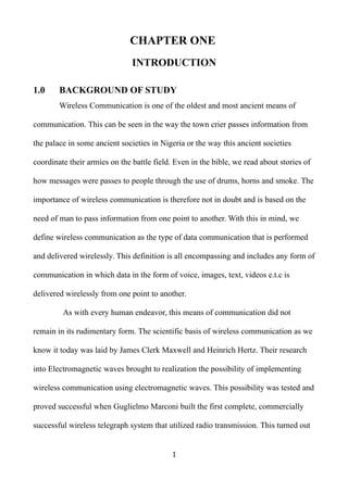
  • 39. 3.1.2 GLOBAL POSITIONING SYSTEM DEVICE This is a small hand held device used for taking measurement of distances covered. This device also gave use the ability to obtain the longitude and latitudes of the base station and each of the points where we stood to take our data. This device is small and easy to use. Fig 3.7: Global Positioning System handheld device 39
  • 40. 3.2 METHODOLOGY In carrying out this research, we went to the city of Warri and located three GSM base stations we would be taking our data from. This process involved the use of the Google maps and NETMONITOR apps which helped us to locate all the surrounding base stations in our area of choice and make our choice on which of them we would be measuring our data. Next we had to physically identify these base stations and made sure its Cell identifying digits (CID) code corresponds with what we are having on our maps. This particular reason lead us to using base stations belonging to MTN Nigeria. All the base station belonging to the company in Warri and environs are all labelled with their logo and the CID number. After we have physically identified the base stations of our choice, we recorded their coordinates and took readings for each of them at every hundred meters for a distance of one thousand five hundred kilometers. This distance was chosen because theoritically, it is the largest radius of a cell in a cellular network. We made sure our distances from the base station was accurately measured with our GPS device, standing at every hundred meters to take our readings from the NETMONITOR app and record it. This process, aside from the base station location and identification, had to be repeated twice every week for two months the months of june and july in other for us to accurately obtain the received signal strength in our areas of study. 3.3 PRESENTATION OF RESULTS The received signal strength (in dBm) for each of the location of study and for each month is presented below in the following tables. 40
  • 41. MONTH OF JUNE Bulos Hotel, Refinery Road (MTN 53212/1532) First Readings Table 3.0: Showing the Received Signal Strength at intervals of 100 meters 41 Distance(m) R.S.S.1 (dBm) R.S.S.2 (dBm) R.S.S.3 (dBm) R.S.S.4 (dBm) Mean 0 -67 -70 -66 -67 -67.5 100 -51 -58 -52 -52 -53.25 200 -65 -67 -65 -63 -65 300 -67 -65 -66 -64 -65.5 400 -73 -69 -70 -69 -70.25 500 -63 -69 -67 -68 -66.75 600 -61 -67 -69 -70 -60 700 -75 -79 -76 -75 -76.25 800 -79 -71 -69 -72 -72.75 900 -76 -67 -69 -70 -70.5 1000 -73 -75 -73 -79 -75 1100 -69 -71 -65 -68 -68.25 1200 -71 -69 -68 -70 -69.5 1300 -79 -75 -71 -81 -76.5 1400 -77 -79 -78 -80 -78.5 1500 -79 -83 -81 -82 -81.25
  • 42. Second Readings Table 3.1: Showing the Received Signal Strength at intervals of 100 meters 42 Distance(m) R.S.S.1 (dBm) R.S.S.2 (dBm) R.S.S.3 (dBm) R.S.S.4 (dBm) Mean 0 -63 -71 -65 -67 -66.5 100 -51 -59 -52 -52 -53.5 200 -63 -53 -57 -55 -57 300 -59 -57 -58 -59 -58.25 400 -63 -61 -68 -65 -64.25 500 -75 -67 -69 -68 -69.75 600 -71 -69 -79 -59 -69.5 700 -65 -69 -59 -70 -65.75 800 -69 -67 -65 -66 -66.75 900 -75 -73 -71 -72 -72.75 1000 -71 -69 -63 -70 -68.25 1100 -75 -77 -81 -80 -78.25 1200 -73 -77 -71 -69 -72.5 1300 -71 -69 -73 -75 -72 1400 -83 -81 -77 -79 -80 1500 -75 -77 -81 -80 -78.25
  • 43. Enerhen (MTN 63216/29013) First Reading Table 3.2: Showing the Received Signal Strength at intervals of 100 meters 43 Distance (m) R.S.S.1 (dBm) R.S.S.2 (dBm) R.S.S.3 (dBm) R.S.S.4 (dBm) Mean 0 -65 -69 -66 -67 -66.75 100 -69 -68 -64 -70 -67.75 200 -81 -85 -83 -84 -83.25 300 -73 -71 -69 -73 -71.5 400 -75 -73 -70 -69 -71.75 500 -80 -82 -81 -82 -81.25 600 -79 -80 -78 -81 -79.5 700 -85 -84 -83 -86 -84.5 800 -82 -83 -81 -79 -81.25 900 -84 -85 -83 -80 -83 1000 -83 -82 -81 -85 -82.75 1100 -82 -81 -84 -85 -83 1200 -83 -84 -82 -81 -82.5 1300 -87 -87 -86 -87 -86.75 1400 -85 -86 -84 -88 -85.75 1500 -84 -85 -85 -83 -84.25
  • 44. Second Reading Table 3.3: Showing the Received Signal Strength at intervals of 100 meters 44 Distance (m) R.S.S.1 (dBm) R.S.S.2 (dBm) R.S.S.3 (dBm) R.S.S.4 (dBm) Mean 0 -51 -52 -55 -53 -52.75 100 -53 -51 -52 -53 -52.25 200 -51 -55 -53 -54 -53.25 300 -71 -69 -67 -65 -68 400 -71 -75 -70 -72 -72 500 -85 -79 -80 -81 -81.25 600 -79 -80 -78 -81 -79.5 700 -85 -84 -83 -86 -84.5 800 -82 -83 -81 -79 -81.25 900 -84 -85 -83 -80 -83 1000 -83 -82 -81 -85 -82.75 1100 -82 -81 -84 -85 -83 1200 -83 -84 -82 -81 -82.5 1300 -87 -87 -86 -87 -86.75 1400 -85 -86 -84 -88 -85.75 1500 -84 -85 -85 -83 -84.25
  • 45. Okuokokor (MTN 63217/27183) First Reading Table 3.4: Showing the Received Signal Strength at intervals of 100 meters 45 Distance (m) R.S.S.1 (dBm) R.S.S.2 (dBm) R.S.S.3 (dBm) R.S.S.4 (dBm) mean 0 -51 -51 -52 -55 -52.25 100 -55 -51 -53 -52 -52.75 200 -55 -51 -52 -53 -52.75 300 -53 -59 -63 -58 -58.25 400 -59 -69 -65 -67 -65 500 -71 -75 -79 -67 -73 600 -71 -67 -79 -67 -71 700 -71 -69 -75 -67 -70.5 800 -65 -69 -71 -70 -68.75 900 -71 -73 -75 -73 -73 1000 -79 -82 -81 -82 -81 1100 -81 -75 -83 -82 -80.25 1200 -80 -79 -81 -82 -80.5 1300 -82 -80 -81 -83 -81.5 1400 -83 -82 -84 -81 -82.5 1500 -84 -81 -83 -85 -83.25
  • 46. Second Reading Table 3.5: Showing the Received Signal Strength at intervals of 100 meters 46 Distance(m) R.S.S.1 (dBm) R.S.S.2 (dBm) R.S.S.3 (dBm) R.S.S.4 (dBm) Mean 0 -55 -52 -51 -51 -52.25 100 -52 -53 -55 -51 -52.75 200 -53 -52 -55 -51 -52.75 300 -58 -63 -53 -59 -58.25 400 -67 -65 -59 -69 -65 500 -67 -79 -71 -75 -73 600 -67 -79 -71 -67 -71 700 -67 -75 -71 -69 -70.5 800 -70 -71 -65 -69 -68.75 900 -73 -75 -71 -73 -73 1000 -82 -81 -79 -82 -81 1100 -82 -83 -81 -75 -80.25 1200 -82 -81 -80 -79 -80.5 1300 -83 -81 -82 -80 -81.5 1400 -81 -84 -83 -82 -82.5 1500 -85 -83 -84 -81 -83.25
  • 47. MONTH OF JULY Bulos Hotel, Refinery Road (MTN 53212/1532) First Readings Table 3.6: Showing the Received Signal Strength at intervals of 100 meters 47 Distance (m) R.S.S.1 (dBm) R.S.S.2 (dBm) R.S.S.3 (dBm) R.S.S.4 (dBm) Mean 0 -60 -71 -64 -68 -65.75 100 -51 -58 -54 -50 -53.25 200 -65 -65 -70 -63 -65.75 300 -60 -67 -66 -64 -64.25 400 -70 -69 -80 -79 -74.5 500 -63 -69 -67 -75 -68.5 600 -61 -66 -60 -70 -64.25 700 -75 -79 -76 -75 -76.25 800 -79 -71 -69 -72 -72.75 900 -73 -64 -65 -70 -68 1000 -74 -75 -63 -79 -72.75 1100 -68 -72 -66 -67 -68.25 1200 -72 -68 -67 -71 -69.5 1300 -79 -75 -72 -82 -77 1400 -70 -79 -78 -80 -76.75 1500 -80 -84 -81 -70 -78.75
  • 48. Second Readings Table 3.7: Showing the Received Signal Strength at intervals of 100 meters 48 Distance(m) R.S.S.1 (dBm) R.S.S.2 (dBm) R.S.S.3 (dBm) R.S.S.4 (dBm) mean 0 -70 -66 -67 -67 -67.5 100 -58 -52 -51 -52 -53.25 200 -67 -65 -65 -63 -65 300 -65 -66 -67 -64 -65.5 400 -69 -70 -73 -69 -70.25 500 -69 -67 -63 -68 -66.75 600 -67 -69 -61 -70 -66.75 700 -79 -76 -75 -75 -76.25 800 -71 -69 -69 -72 -70.25 900 -76 -67 -69 -70 -70.5 1000 -73 -75 -73 -79 -75 1100 -69 -71 -65 -68 -68.25 1200 -71 -69 -68 -70 -69.5 1300 -79 -75 -71 -81 -76.5 1400 -77 -79 -78 -80 -78.5 1500 -79 -83 -81 -82 -81.25
  • 49. Enerhen (MTN 63216/29013) First Readings Table 3.8: Showing the Received Signal Strength at intervals of 100 meters 49 Distance(m) R.S.S.1(dBm) R.S.S.2(dBm) R.S.S.3(dBm) R.S.S.4(dBm) mean 0 -65 -66 -55 -69 -63.75 100 -69 -64 -52 -68 -63.25 200 -81 -83 -53 -85 -75.5 300 -73 -69 -67 -71 -70 400 -75 -70 -70 -73 -72 500 -80 -81 -80 -82 -80.75 600 -79 -78 -78 -81 -79 700 -85 -84 -83 -86 -84.5 800 -82 -83 -81 -79 -81.25 900 -84 -85 -83 -80 -83 1000 -83 -82 -81 -85 -82.75 1100 -82 -81 -84 -85 -83 1200 -83 -84 -82 -81 -82.5 1300 -87 -87 -86 -87 -86.75 1400 -85 -86 -84 -88 -85.75 1500 -84 -85 -85 -83 -84.25
  • 50. Second Readings Table 3.9: Showing the Received Signal Strength at intervals of 100 meters 50 Distance(m) R.S.S.1(dBm) R.S.S.2(dBm) R.S.S.3(dBm) R.S.S.4(dBm) mean 0 -65 -66 -55 -69 -63.75 100 -69 -64 -52 -68 -63.25 200 -81 -83 -53 -85 -75.5 300 -73 -69 -67 -71 -70 400 -75 -70 -70 -73 -72 500 -80 -81 -80 -82 -80.75 600 -79 -78 -78 -81 -79 700 -85 -84 -83 -86 -84.5 800 -82 -83 -81 -79 -81.25 900 -84 -85 -83 -80 -83 1000 -83 -82 -81 -85 -82.75 1100 -82 -81 -84 -85 -83 1200 -83 -84 -82 -81 -82.5 1300 -87 -87 -86 -87 -86.75 1400 -85 -86 -84 -88 -85.75 1500 -84 -85 -85 -83 -84.25
  • 51. Okuokokor (MTN 63217/27183) First Readings Table 3.10: Showing the Received Signal Strength at intervals of 100 meters 51 Distance(m) R.S.S.1(dBm) R.S.S.2(dBm) R.S.S.3(dBm) R.S.S.4(dBm) mean 0 -52 -53 -54 -55 -53.5 100 -50 -50 -53 -52 -51.25 200 -52 -51 -56 -57 -54 300 -56 -59 -60 -58 -58.25 400 -59 -69 -65 -67 -65 500 -71 -75 -79 -67 -73 600 -72 -65 -78 -66 -70.25 700 -73 -69 -75 -67 -71 800 -65 -69 -71 -70 -68.75 900 -71 -73 -75 -77 -74 1000 -80 -81 -81 -82 -81 1100 -81 -73 -82 -82 -79.5 1200 -80 -79 -82 -82 -80.75 1300 -82 -80 -83 -83 -82 1400 -83 -82 -81 -81 -81.75 1500 -89 -81 -85 -85 -85
  • 52. Second Readings Table 3.11: Showing the Received Signal Strength at intervals of 100 meters The summary of the above table showing the average of the values obtained for each of the locations for the months during which the study was carried out is shown below. 52 Distance(m) R.S.S.1(dBm) R.S.S.2(dBm) R.S.S.3(dBm) R.S.S.4(dBm) mean 0 -52 -55 -52 -55 -53.5 100 -53 -52 -53 -52 -52.5 200 -52 -53 -52 -53 -52.5 300 -63 -58 -63 -58 -60.5 400 -65 -67 -65 -67 -66 500 -79 -67 -79 -67 -73 600 -79 -67 -79 -67 -73 700 -75 -67 -75 -67 -71 800 -71 -70 -71 -70 -70.5 900 -75 -73 -75 -71 -73.5 1000 -81 -82 -81 -79 -80.75 1100 -83 -82 -83 -81 -82.25 1200 -81 -82 -81 -80 -81 1300 -81 -83 -81 -82 -81.75 1400 -84 -81 -84 -83 -83 1500 -83 -85 -83 -84 -83.75
  • 53. MONTH OF JUNE Table 3.12: Showing the Average of all the values obtained 53 Distance (m) Refinery Road Enerhen Okuokorkor 0 -67 -68.375 -52.25 100 -53.375 -60 -52.75 200 -61 -68.25 -52.75 300 -61.875 -69.75 -58.25 400 -67.25 -71.875 -65 500 -68.25 -81.25 -73 600 -64.75 -79.5 -71 700 -71 -84.5 -70.5 800 -69.75 -81.25 -68.75 900 -71.625 -83 -73 1000 -71.625 -82.75 -81 1100 -73.25 -83 -80.25 1200 -71 -82.5 -80.5 1300 -74.25 -86.75 -81.5 1400 -79.25 -85.75 -82.5 1500 -79.75 -84.25 -83.25
  • 54. MONTH OF JULY Table 3.13: Showing the Average of all the values obtained 54 Distance (m) Refinery Road Enerhen junction Okuokorkor 0 -66.625 -63.75 -53.5 100 -53.25 -63.25 -51.875 200 -65.375 -75.5 -53.25 300 -64.875 -70 -59.375 400 -72.375 -72 -65.5 500 -67.625 -80.75 -73 600 -65.5 -79 -71.625 700 -76.25 -84.5 -71 800 -71.5 -81.25 -69.625 900 -69.25 -83 -73.75 1000 -73.875 -82.75 -80.875 1100 -68.25 -83 -80.875 1200 -69.5 -82.5 -80.875 1300 -76.75 -86.75 -81.875 1400 -77.625 -85.75 -82.375 1500 -80 -84.25 -84.375
  • 55. 3.4 CALCULATIONS Before we begin our calculations proper, a summary of the antenna properties are provided below. Table 3.14: Transmitting Antenna Parameter Refinery Road Enerhen Road Okuokokor Antenna Heights (M) 33 20 52 Transmitting Frequency (MHz) 900 900 900 Transmitting Power (Watts) 40 40 40 Antenna’s Gain (dBi) 17.5 17.5 17.5 VSWR (Voltage Standing Wave Ratio) 1.5 1.5 1.5 In order for us to be able to calculate the path-loss, we have to calculate the for the Effective Isotropic Radiated Power (EIRP) which is given by the formula below EIRP = Pout - RL + Gt where Pout = The transmitter power output in dBm RL = Signal loss in cable (dB) Gt = Gain of the antenna (dBi) Now, RL = 20 log10 VSWR+1 VSWR−1 dB Since all of the antennas at the various locations all have the same VSWR, their return loss values would be the same. This value is calculated below RL = 20 log10 1.5+1 1.5−1 = 13.98 dB The ouput power which is given in watts has to be converter to Decibel milliwatts 55
  • 56. (dBm) before it can be used in the equation. Therefore, the formula for convertion of power in watts to Decibel milliwatts is given below dBm = 10log 1000∗power inwatts 1milliwatts = 10log (1000∗40)mW 1mW = 46.02 dBm therefore, the EIRP for the antenna at Refinery road is given as EIRP = 46.02 - 13.98 + 17.5 = 49.54 dBm At Enerhen junction, EIRP = 46.02 - 13.98 + 17.5 = 49.54 dBm At Okuokorkor, EIRP = 46.02 - 13.98 + 17.5 = 49.54 dBm Now the path-loss (Pl) is gotten as the difference between the effective Isotropic Radiated Power (EIRP) and the received power (Pr) i.e Pl = EIRP - Pr the results obtained are shown in chapter four. 56
  • 57. 3.4.1 PATH-LOSS USING Free-space MODEL The formula for the free-space path-loss is as shown below Path-loss = 20log10 (d) + 20log10 (f) – 27.55 (Rappaport 2002) Where d = distance in metres f = frequency of operation in megahertz of the antenna given above. = 900MHz This formula gives us the table shown below for all the expected path-loss at each of the study areas for the month of june and july. Table 3.15: Results obtained using the Free-space model 57 Distance (m) Refinery Road Enerhen (in dBm) Okuokokor (in dBm) 0 0 0 0 100 71.53 71.53 71.53 200 77.56 77.56 77.56 300 81.08 81.08 81.08 400 83.58 83.58 83.58 500 85.51 85.51 85.51 600 87.10 87.10 87.10 700 88.44 88.44 88.44 800 89.60 89.60 89.60 900 90.62 90.62 90.62 1000 91.53 91.53 91.53 1100 92.36 92.36 92.36 1200 93.12 93.12 93.12 1300 93.81 93.81 93.81 1400 94.46 94.46 94.46 1500 95.06 95.06 95.06
  • 58. 3.4.2 PATH-LOSS USING OKUMURA-HATA MODEL Using the formula shown below for the Okumura-Hata model, we obtained the results shown for the three locations. PL = A + B log(d) + C Where A = 69.55 + 26.16 log(fc) − 13.82 log(hb) − a(hm) B = 44.9 − 6.55 log(hb) Where fc is given in MHz and it is the operating frequency of the antenna which is 900MHz at all the locations under study. d in km. hm is the height of the mobile station in meters which in this case is 1m. hb is the height of the base station antenna which is 20m at Enerhen junction, 33m at Refinery Road and 52m at Okuokorkor. The function a(hm) and the factor C depend on the environment So For Refinery Road, a(hm) = (1.1 log(fc) − 0.7)hm − (1.56 log(fc) − 0.8) = -1.259 C = 0 A = 69.55 + 26.16 log(fc) − 13.82 log(hb) + 1.259 = 127.106 B = 44.9 − 6.55 log(hb) = 34.9536 For Enerhen Junction, a(hm) = 3.2(log(11.75hm))2 − 4.97 = -1.306 C = 0 A = 69.55 + 26.16 log(fc) − 13.82 log(hb) + 1.306 58
  • 59. = 130.159 B = 44.9 − 6.55 log(hb) = 36.38 For Okuokorkor, a(hm) = (1.1 log(fc) − 0.7)hm − (1.56 log(fc) − 0.8) = -1.259 C = 0 A = 69.55 + 26.16 log(fc) − 13.82 log(hb) + 1.259 = 124.377 B = 44.9 − 6.55 log(hb) = 33.66 Having gotten the necessary parameters needed to solve for the path-loss at each of the locations, we can now solve for the path-loss at each of these locations. This computation was done using the LibreOffice Calc spreadsheet software and the results obtained are presented in chapter 4. 59
  • 60. CHAPTER FOUR DISCUSSION AND FINDINGS 4.0 INTRODUCTION In this chapter, the results obtained from the previous chapter would be explained and insights gained in that chapter would be noted and also explained here. 4.1 DISCUSSION OF RESULTS The result of the calculations done in section 3.4 to obtain the Measured path- loss from the areas under study is shown below Table 4.0: Results obtained from section 3.4 for the Measured path-loss for the Month of June 60 Distance (m) Refinery Road (in dBm) Enerhen (in dBm) Okuokokor (in dBm) 0 116.54 117.92 101.77 100 102.92 109.54 102.27 200 110.54 117.79 102.27 300 111.42 119.29 107.77 400 116.79 121.42 114.52 500 117.79 130.79 122.52 600 114.29 129.04 120.52 700 120.54 134.04 120.02 800 119.29 130.79 118.27 900 121.17 132.54 122.52 1000 121.17 132.29 130.52 1100 122.79 132.54 129.77 1200 120.54 132.04 130.02 1300 123.79 136.29 131.02 1400 128.79 135.29 132.02 1500 129.29 133.79 132.77
  • 61. Month of July This shows that the acquired data was sufficient in sampling the amount of path-loss obtained in this area. From the results obtained above, there is a general increase of the path-loss with respect to distance. This increase however is not strictly linear with cases of the path-loss values at distances closer to the base station being larger than values obtained at distances far from it. This is due partial to the uneven distribution of substances that can increase the path-loss of the signal. At Enerhren junction, we find that the path-loss was already above 130 dBm at a distance of 700 m from the base station with a variation of + 4 dBm for each subsequent increase of about 100 m till we get to 1500 m. At refinery road, the results obtained is generally lower than that obtained at enerhen junction with the maximum path-loss obtained being 129 61 Distance (m) Refinery Road (in dBm) Enerhen (in dBm) Okuokokor (in dBm) 0 116.17 113.29 103.02 100 102.79 112.79 101.40 200 114.92 125.04 102.77 300 114.42 119.54 108.90 400 121.92 121.54 115.02 500 117.17 130.29 122.52 600 115.04 128.54 121.15 700 125.79 134.04 120.52 800 121.04 130.79 119.15 900 118.79 132.54 123.27 1000 123.42 132.29 130.40 1100 117.79 132.54 130.40 1200 119.04 132.04 130.40 1300 126.29 136.29 131.40 1400 127.17 135.29 131.90 1500 129.54 133.79 133.90
  • 62. dBm but this result was still subject to the exact type of variations that occurred with the previous case with the values hovering around 120 dBm for much of the distances covered. Finally, the maximum values obtained for Okuokorkor was similar to Enerhen junction but this values was not constant until we were at distances above 1100 m. Note the value of zero was used as the first entry in the table above because the log of zero is negative infinity and our answer would be just that. The Free-space model, which was used to calculate for the path-loss in section 3.4.1, produced the table shown below Table 4.1: Free-space Model Predicted Path-loss This results obtained shows that irrespective of the environment, the results 62 Distance (m) Refinery Road Enerhen (in dBm) Okuokokor (in dBm) 0 0 0 0 100 71.53 71.53 71.53 200 77.56 77.56 77.56 300 81.08 81.08 81.08 400 83.58 83.58 83.58 500 85.51 85.51 85.51 600 87.10 87.10 87.10 700 88.44 88.44 88.44 800 89.60 89.60 89.60 900 90.62 90.62 90.62 1000 91.53 91.53 91.53 1100 92.36 92.36 92.36 1200 93.12 93.12 93.12 1300 93.81 93.81 93.81 1400 94.46 94.46 94.46 1500 95.06 95.06 95.06
  • 63. obtained for the predicted path-loss values would always be the same. This results also shows that for the specified maximum distance which is 1500 m the predicted path-loss would always be the same for the three locations which is 95.06 dBm. It is also observed from the results above that there is a gradual increase in the predicted path-loss with each increase in distance. That is as we increase the distance, the predicted path-loss must increase. This is due to the fact that the predicted path-loss is a function of transmitting frequency and distance and since the transmitting frequency is the same, the change is as a result of change in distance only. Table 4.2: Difference between the Measured Path-loss and Free-space Path-loss for the Month of June 63 Distance (m) Refinery Road Enerhen Junction Okuokorkor 0 116.54 117.92 101.77 100 31.38 38.01 30.74 200 32.98 40.23 24.71 300 30.34 38.21 26.69 400 33.21 37.84 30.94 500 32.28 45.28 37.01 600 27.19 41.94 33.42 700 32.10 45.60 31.58 800 29.69 41.19 28.67 900 30.55 41.92 31.90 1000 29.63 40.76 38.99 1100 30.43 40.18 37.41 1200 27.42 38.92 36.90 1300 29.98 42.48 37.21 1400 34.33 40.83 37.56 1500 34.23 38.73 37.71
  • 64. Table 4.3: Difference between the Measured Path-loss and Free-space Path-loss for the Month of July For the Okumura-Hata model, the results obtained from the calculations done in section 3.4.2 is shown in the table below 64 Distance (m) Refinery Road Enerhen Junction Okuokorkor 0 116.17 113.29 103.02 100 31.26 41.26 29.86 200 37.36 47.48 25.21 300 33.34 38.46 27.82 400 38.34 37.96 31.44 500 31.65 44.78 37.01 600 27.94 41.44 34.05 700 37.35 45.60 32.08 800 31.44 41.19 29.55 900 28.17 41.92 32.65 1000 31.88 40.76 38.86 1100 25.43 40.18 38.03 1200 25.92 38.92 37.28 1300 32.48 42.48 37.58 1400 32.71 40.83 37.44 1500 34.48 38.73 38.84
  • 65. Table 4.4: Okumura-Hata Predicted Path-loss The values obtained from this model shows that the environment was taken into consideration in this model. The values obtained for refinery road was distinctively different from that obtained for enerhen junction and okuokorkor. 65 Distance (km) Refinery Road Enerhen Junction Okuokorkor 0 0 0 0 0.1 92.15 93.78 90.72 0.2 102.67 104.73 100.85 0.3 108.83 111.14 106.78 0.4 113.20 115.68 110.98 0.5 116.58 119.21 114.24 0.6 119.35 122.09 116.91 0.7 121.69 124.52 119.16 0.8 123.72 126.63 121.12 0.9 125.51 128.49 122.84 1 127.11 130.16 124.38 1.1 128.55 131.66 125.77 1.2 129.87 133.04 127.04 1.3 131.09 134.30 128.21 1.4 132.21 135.48 129.30 1.5 133.26 136.57 130.30
  • 66. Table 4.5: Difference between the Measured Path-loss and Okumura-Hata Path- loss for the Month of June 66 Distance (m) Refinery Road Enerhen Junction Okuokorkor 0 116.54 117.92 101.77 100 10.76 15.76 11.55 200 7.87 13.06 1.42 300 2.59 8.15 0.99 400 3.59 5.73 3.54 500 1.21 11.58 8.28 600 -5.06 6.95 3.61 700 -1.15 9.52 0.86 800 -4.43 4.16 -2.85 900 -4.34 4.05 -0.32 1000 -5.94 2.13 6.14 1100 -5.76 0.88 4.00 1200 -9.33 -1.00 2.98 1300 -7.30 1.99 2.81 1400 -3.42 -0.19 2.72 1500 -3.97 -2.78 2.47
  • 67. Table 4.6: Difference between the Measured Path-loss and Okumura-Hata Path- loss for the Month of July 67 Distance (m) Refinery Road Enerhen Junction Okuokorkor 0 116.17 113.29 103.02 100 10.64 19.01 10.68 200 12.24 20.31 1.92 300 5.59 8.40 2.12 400 8.72 5.86 4.04 500 0.58 11.08 8.28 600 -4.31 6.45 4.24 700 4.10 9.52 1.36 800 -2.68 4.16 -1.97 900 -6.72 4.05 0.43 1000 -3.69 2.13 6.02 1100 -10.76 0.88 4.62 1200 -10.83 -1.00 3.35 1300 -4.80 1.99 3.18 1400 -5.05 -0.19 2.60 1500 -3.72 -2.78 3.59
  • 68. The results obtained through the various methods at different locations are presented in the graphs shown below. The graph of the results obtained at Refinery road comparing their values are shown below. Fig 4.0: Graphical Representation of the values obtained at Refinery Road for June 68
  • 69. Fig 4.1: Graphical Representation of the values obtained at Refinery Road for July 69
  • 70. The graph above shows us graphically that the Okumura-Hata model was fairly accurate at predicting the Path-loss to be expected at this location. Comparing it with the Measured Path-loss, the results shows us that both values intersects at more that four points with the other Measured values being either above or below the values predicted by the Okumura-Hata model. The Free-space model on the other hand was very far from the Measured values. The graph of the values obtained at Enerhen junction is presented below. Fig 4.2: Graphical Representation of the values obtained at Enerhen Junction for June 70
  • 71. Fig 4.3: Graphical Representation of the values obtained at Enerhen Junction for July From the graphs above, both lines representing the Measured values and the Okumura-Hata model intersected at different points with the remaining values being very close. This is obvious that the Measured Values settles for the predicted values obtained from the Okumura-Hata model as the range of the distance is increased. It is also obvious that the Free-space model is still not performing well when compared with the other two method. Lastly, the graphical representation of the values obtained at Okukorkor is presented below 71
  • 72. Fig 4.4: Graphical Representation of the values obtained at Okuokorkor for the Month of June Fig 4.5: Graphical Representation of the values obtained at Okuokorkor for the Month of July 72
  • 73. This values shows that the Okumura-Hata model still maintained its high performance and intergrity. It was still very close to the Measured value, ignoring the fact that they both intersected at a single point. The okumura-Hata model performed well in trying to predict the path-loss in this area. In general, the Okumura-Hata model performed well in trying to predict the Path-loss in Warri and its environs. Fig 4.6: Graphical Representation of the Difference between the Measured Path-loss and Free-space Path-loss for the Month of June 73
  • 74. Fig 4.7: Graphical Representation of the Difference between the Measured Path-loss and Free-space Path-loss for the Month of July 74
  • 75. Fig 4.8: Graphical Representation of the Difference between the Measured Path-loss and Okumura-Hata Path-loss for the Month of June 75
  • 76. Fig 4.9: Graphical Representation of the Difference between the Measured Path-loss and Okumura-Hata Path-loss for the Month of July 76
  • 77. 4.2 Findings Firstly, we discovered that the Okumura-Hata model was very good at giving a good estimate of the path-loss at the areas under consideration. The accuracy of the path-loss gotten through this model when compared with the free-space model only got better as the distance from the base station is increased. It is also very close to the measured path-loss obtained from measurements. This shows us that the Okumura- Hata model can be used as an alternative to calculate for the path-loss in this areas if the cost of carrying out experiments and the time involved is not acceptable. Secondly, it was observed that the measured path-loss, as seen from the graph, usually settles for the same value as the Okumura-Hata model as the distance increases. This also adds to the already high reliability of the Okumura-Hata model. Lastly, the free-space model was shown to be highly unreliable as shown in the graphs above. This model did not predict any value close to the Measured or Okumura-Hata values. This shows that the Free-space model cannot be relied upon at any distance or in any environment to accurately predict the signal path-loss. 77
  • 78. CHAPTER FIVE CONCLUSION AND RECOMMENDATION 5.0 CONCLUSION In line with the aim of this study, it has been proven practically, through this study, that the Okumura-Hata model is very accurate in its prediction of the path-loss in Warri and its environs. This study also showed that the free-space model is very inaccurate in its prediction of the path-loss experienced in Warri. It is to be noted that despite the accuracy of this model in predicting the path- loss in this environment, the results obtained in this research is subject to changes due to the ever changing nature of our environment. This changes can be natural or man- made, permanent or temporary, instant or gradual. It should also be noted that these two models are not the only models that can be used to predict the path-loss in an environment like Warri. The Okumura-Hata model has proven to be very reliable and accurate in its prediction of path-loss encountered and it is recommended as a suitable replacement to taking exact measurements if the cost in time, money and effort is too great to bear. 5.1 RECOMMENDATION 1. We recommend that further research be carried out in Warri and its environs, comparing the accuracy of other prediction models and comparing it with that of the already established Okumura-Hata model. 2. We recommend also that the readings acquired during the cause of this study 78
  • 79. be reaccessed after a couple of years due to the ever changing nature of the environment as stated above. 3. The Free-space model should not be used as the major prediction model in any practical work. 79
  • 80. REFERENCES Obot .A, O. Simeon and J. Afolayan (2011), “Comparative analysis of path loss prediction models for urban macrocellular environments”, Nigerian Journal of Technology, Vol. 30, No. 3 Andrea Goldsmith, “Wireless Communications,” Cambridge University Press, Andreas.F. Molish (2011), “Wireless Communication,” John Wiley & Sons Ltd, The Atrium, Southern Gate, Chichester, West Sussex, PO19 8SQ, United Kingdom. Daniel .K Wong, (2012) “Fundamentals of Wireless Communication Engineering Technologies,” John Wiley & Sons, Inc., Hoboken, New Jersey. Isabona Joseph, Konyeha. C. C, Chinule. C. Bright, and Isaiah Gregory Peter (2013), “Radio Field Strength Propagation Data and Path-loss calculation Methods in UMTS Network”, Advances in Physics Theories and Applications ISSN 2224-719X (Paper) ISSN 2225-0638 (Online) Vol.21 Nasir Faruk, Adeseko A. Ayeni and Yunusa A. Adediran (2013),”On the study of empirical path loss models for accurate prediction of tv signal for secondary users”, Progress In Electromagnetics Research B, Vol. 49, 155–176 Nwalozie gerald .C, Ufoaroh S.U, Ezeagwu C.O and Ejiofor A.C (2014),”Path loss prediction for GSM mobile networks for urban region of aba, south-east Nigeria”, International Journal of Computer Science and Mobile Computing, Vol.3 Issue.2, pg. 267-281. Theodore S. Rappaport (2002)“Wireless Communications: Principles and Practice”, Prentice Hall Ubom, E.A., Idigo, V. E., Azubogu, A.C.O., Ohaneme, C.O., and Alumona, T. L (2011) “Path loss Characterization of Wireless Propagation for South -South Region of Nigeria”, International Journal of Computer Theory and Engineering, Vol. 3, No. 3 80
  • 81. Williams Stallings, (2005) “Wireless Communication and Network,” Pearson Education Inc, Upper Saddle River, NJ 07458. 81