ISOQUANTS OR EQUAL PRODUCT CURVES

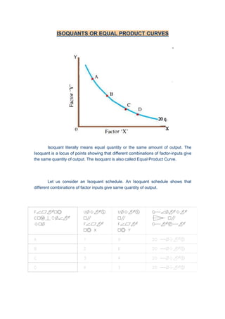
1. ISOQUANTS OR EQUAL PRODUCT CURVES
Isoquant literally means equal quantity or the same amount of output. The
Isoquant is a locus of points showing that different combinations of factor-inputs give
the same quantity of output. The Isoquant is also called Equal Product Curve.
Let us consider an Isoquant schedule. An Isoquant schedule shows that
different combinations of factor inputs give same quantity of output.
Factor
Combinat
ion
Units
of
Fact
or X
Units
of
Fact
or Y
Quantit
y of
Output
A 1 9 20 units
B 2 6 20 units
C 3 4 20 units
D 4 3 20 units

2. Let us plot the graph with factor X shown on the X-axis and factor Y on the
Y-axis. Plotting the factor combinations; viz. points A, B, C and D respectively and
joining these points we get the curve. This is an Isoquant representing 20 units of
output.
Thus different points on the same Isoquant curve show that different factor
combinations can be used to yield the same quantity of output. Therefore Isoquant
curve is also called the equal-product curve.
Thus an Isoquant is a curve any point on which shows that various
combinations of factor inputs yield the same level of output. At this stage it may be
noted that as the Isoquant represents the level of output and as output is physically
quantifiable the Isoquant must be labeled not only as just IQ but must represent the
quantity produced e.g. 20q. The Isoquant thus labeled as 20q shows all possible
combinations of factors that yield 20 units of output at any point on that curve.
Marginal Rate of Technical Substitution
Since with different factor-combinations we are able to produce same quantity
of output it necessarily implies that factors of production are substitutes to each other;
for if factor-inputs were not substitutes then we would not have obtained the same
level of output. Thus the Isoquant implies factor substitutability. The factors need not
be perfect substitutes but they do possess an element of substitutability e.g. if 1x+9y
can produce 20q and 2x+6y can also produce 20q, then it implies that 3 units of input
Y are substituted by 1 unit of input X, so as to yield the same level of output.
The rate at which one factor-input is substituted by the other is called the Rate
of Technical Substitution. To obtain the Marginal Rate of Technical Substitution
(MRTS) we try to find out as to how many units of input Y are substituted by one
additional unit of factor input X. combination A of 1X + 9Y yields 20q ; and
combination B of 2X + 6Y also yields the same quantity of output viz. 20q, one unit of
factor X can displace 3 units of factor Y. hence the MRTS is 3:1
MRTS = ΔX/ΔY

3. Factor Combin
ation
Units
of Fac
tor X
Units
of Fac
tor
Y
MRT
S
=
?Y
/?
X
A 1 9 —-
B 2 6 3:1
C 3 4 2:1
D 4 3 1:1
It is important to note that the MRTS goes on diminishing. This gives rise to
the Principle of Diminishing Marginal Rate of Technical Substitution.
Properties of Isoquants
1. An Isoquant must slope downward from left to right. The logic behind this is the
principle of diminishing marginal rate of technical substitution. In order to maintain
a given output, a reduction in the use of one input must be offset by an increase in
the use of another input.
2. Isoquant must be convex to the point of origin. This is because of the operation of
the principle of diminishing marginal rate of technical substitution. MRTS is the
rate at which marginal unit of an input can be substituted for another input making
the level of output remain the same.
3. No two Isoquants should intersect each other. Just as two indifference curves
cannot cut each other, two isoquants also cannot cur each other. If they intersect
each other, there would be a contradiction and we will get inconsistent results.
4. Isoquants need not be parallel. The shape of an isoquant depends upon the
marginal rate of technical substitution. Since the rate of substitution between two
factors need not necessarily be the same in all the isoquant schedules, they need
not be parallel.