- A system is at static equilibrium when it is at rest and experiences no translation or rotation (according to Newton's 1st law). The net external forces and torques on the system must equal zero. - Dynamic equilibrium applies to accelerating rigid bodies (according to Newton's 2nd law). The net external forces must equal mass times acceleration, and net torque must equal moment of inertia times angular acceleration. - Inverse dynamics uses measured joint positions, ground reaction forces, and segment parameters to compute unknown joint forces and torques that produce the observed motion. Segments are analyzed individually from distal to proximal.

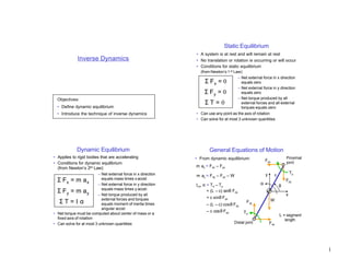
1. Static Equilibrium
• A system is at rest and will remain at rest
Inverse Dynamics • No translation or rotation is occurring or will occur
• Conditions for static equilibrium
(from Newton’s 1 st Law):
– Net external force in x direction
Σ Fx = 0 equals zero
– Net external force in y direction
Σ Fy = 0 equals zero
Objectives: – Net torque produced by all
ΣT=0 external forces and all external
• Define dynamic equilibrium torques equals zero
• Introduce the technique of inverse dynamics • Can use any point as the axis of rotation
• Can solve for at most 3 unknown quantities
Dynamic Equilibrium General Equations of Motion
• Applies to rigid bodies that are accelerating • From dynamic equilibrium: Proximal
Fpx joint
• Conditions for dynamic equilibrium
(from Newton’s 2nd Law): m ax = Fdx – Fpx
– Net external force in x direction y Tp
m ay = Fdy – Fpx – W c
Σ Fx = m a x equals mass times x accel.
α
Fpy
– Net external force in y direction Icm α = Td – Tp θ
Σ Fy = m a y – equals mass times y accel.
Net torque produced by all
+ (L – c) sinθ Fdx
x
+ c sinθ Fpx
ΣT=Iα external forces and torques
equals moment of inertia times – (L – c) cos θ Fdy
Fdy W
angular accel.
– c cos θ Fpy Td
• Net torque must be computed about center of mass or a L = segment
fixed axis of rotation length
• Can solve for at most 3 unknown quantities Distal joint Fdx
1

2. Fhipx
Computing Joint Forces and Torques Analysis by Segment Thip
• It is possible to measure: θthigh Fhipy
• To compute joint forces
– joint position (using video / motion capture system; lab 3) and torques, body is Fkneey
– ground reaction forces (using force plate; lab 6) broken down into Wthigh
– center of pressure (using force plate) Fkneex Tknee
individual segments
• From joint position data, can compute: Fkneex
– absolute angle of each body segment (lab 5) • Analyze from distal to Tknee
proximal θleg
– location of center of mass of each segment (lab 8)
• Can use central difference method to compute: Fankley Fkneey
– angular velocity of segment (lab 5) Wleg
– angular acceleration of segment Tankle
Fanklex Tankle Fanklex
– x and y velocity of segment center of mass (lab 3)
– x and y acceleration of segment center of mass
Fgrfx
• Finally, use general equations of motion to compute θfoot
Fankley Fgrfy
joint forces and torques Wfoot
The End
2