Z Score,T Score, Percential Rank and Box Plot Graph
1 d heat equation
1. ONE DIMENSIONAL HEAT EQUATION
2
u u
c2
t x2
Introduction: -A uniform homogenous rod is made of infinite number of molecules. They are
interconnected by cohesive force. When heat is applied to a rod through a one side of it, they tends to
get expand, because of that they gets even more interconnected and hence heat flows molecule to
molecule more rapidly. The flow of heat in this way in a uniform of rod is known as Heat Conduction.
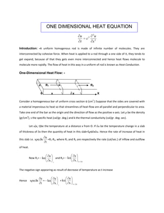
One-Dimensional Heat Flow: -
α R1 R2
0 x x X
Consider a homogeneous bar of uniform cross section α (cm2.) Suppose that the sides are covered with
a material impervious to heat so that streamlines of heat-flow are all parallel and perpendicular to area.
Take one end of the bar as the origin and the direction of flow as the positive x-axis. Let be the density
(gr/cm3), s the specific heat (cal/gr. deg.) and k the thermal conductivity (cal/gr. deg. sec).
Let u(x, t)be the temperature at a distance x from O. If u be the temperature change in a slab
of thickness of x then the quantity of heat in this slab=S α x u. Hence the rate of increase of heat in
u
this slab i.e. s x =R1-R2, where R1 and R2 are respectively the rate (cal/sec.) of inflow and outflow
t
of heat.
u u
Now R1= k and R2= k
x x
x x x
The negative sign appearing as result of decrease of temperature as t increase
u u u
Hence s x = k +k
t x x
x x x
2. u u
u k x x x x x
i.e. =
t s x
k
Writing c 2 , called the diffusivity of the substance (cm2/sec.,) and taking limit x 0, we get
s
2
u 2 u
c is called the one-dimensional Heat-flow equation.
t x2
Solution of One-Dimensional Heat Equation by the method of separating
variables: (with insulated faces)
We first consider the temperature in a long thin bar or thin wire of constant cross section
and homogeneous material, which is oriented along x-axis and is perfectly insulated laterally, so
that heat flows in the x-direction only. Then u depends only on x and time t, and the heat
equation becomes the one-dimensional heat equation
2
u u
c2 -------------------------------------------------(1)
t x2
We take the case that both ends x=0 and x=L are kept at zero degree temperature, we have the
boundary conditions
u(0,t)=0, u(L, t)=0 for all t
-------------------------------(2)
and the temperature in the bar is f(x), so that we have the initial condition
u(x, 0)=f(x)
-------------------------------(3)
Method of separating the variables:
In the method of separating variables or product method, we determine the solution of
Heat equation (1) of the form,
u(x, t)=F(x)G(t)
3. -------------------------------(4)
Where F(x) is only a function of x and G(t) is only a function t only, on differentiating equation
(4), we obtain,
2
u u
FG F "G
t x2
Where dot denotes the partial derivatives with respect to t and primes derivatives with respect to
x. By inserting this into differential equation (1), we get
FG c 2 F "G On dividing by c2FG we obtain,
G F"
c 2G F
The left-hand side the right hand side of the above equation are function t and x respectively and
since both x & t are both independent variables, they must be equal to some constant k=-p2.
We assume k = - p2 because the solution for k =0 and k = p2 is not consistent with the physical
problem i.e. it will not give the transient solution where the temperature decreases as time
inceases.
G F"
k p2
c 2G F
This yields two differential equations, namely
F”+ p2F=0. ----------------------------------------------------------(5)
And
---------------------------------------------------(6)
G p 2 c 2G 0.
Satisfying the boundary conditions: -
Solving (5) the general solution is given by F(x)=Acospx+Bsinpx. ---------(i)
From the boundary (2) it follows that
u(0, t)=F(0)G(t)=0 and u(L, t)=F(L)G(t)=0.
Since G 0 would gives u 0. Which is of no interest. Hence G 0. This gives F(0)=0 and F(L)=0.
4. From (i) F(0)=0 0=A F(x) = B sinpx
F(L)=0 0 = B sin(pL) sin(pL) = 0 ( B 0)
pL = nπ ( zeros of sine)
p = nπ/ L, n=0,1,2,-------
Applying above conditions, we obtain the infinitely many solutions of F(x) are given by
n x
Fn ( x ) B n sin -----------------------------------------------------(7)
L
2
n 2
Solving (6), The constant k is now restricted to the values k=-p =- . Inserting it into the
L
n c
2
equation (6) we get G n G 0 n
L
2
t
Its general solution is given by G n t Cn e n
n 1,2,3- - - - - where Cn is constant. Hence the
functions
n x 2
nt
u n x, t Fn ( x )G n t a n sin e (n 1,2,3 - - - --) where a n Bn C n
L -------(8)
are solutions of the heat equation (1) satisfying (2). These are the Eigenfunctions of the problem,
n c
corresponding to the Eigen values n .
L
Since the equation (1) is linear and homogeneous applying principle of superposition we
obtain the general solution of (1) is given by
n x 2
nt
n c
u x, t u n x, t a n sin e (n 1,2,3 - - - --) where
L ----(9)
n
n 1 n 1 L
Applying (3) on the above equation (9), we obtain
n x
u x ,0 a n sin f x.
n 1 L
So, f(x) is Half-range Fourier series with an’s as Fourier coefficients and is given by
L
2 n x
an f x sin dx ------------------------------------------------------------(10)
L0 L
5. Examples
1. A rod of length l with insulated sides is initially at a uniform temperature u0. Its ends are
suddenly cooled at 00 C and are kept at that temperature. Find the temperature function
u(x,t).
Solution:
The temperature function u(x,t) satisfies the differential equation
u u
c2
t x2
The boundary conditions associated with the problem are
u(0,t)=0, u(l,t)=0
The initial condition is u(x,0)=u0
Its solution is
n x 2
nt
n c
u x, t u n x, t an sin e , n
n 1 n 1 l l
Since u(x,0)=u0 we have
n x
u0 an sin which is the half-range sine series for u0 where
n 1 l
l 0, when n is even
2 n x
an u0 sin dx 4u0
l 0 l , when n is odd
n
Hence the temperature function is
4u0 1 n x c 2 n2 2
t
u ( x, t ) sin e
n 1,3,5,..... n l l2
2. (a) An insulated rod of length l has its ends A and B maintained at 00C and 1000C
respectively until steady state conditions prevail. If B is suddenly reduced to 00C and
maintained at 00C, find the temperature at a distance x from A at time t.
(b) Find also the temperature if the change consists of raising the temperature of A to
200C and that of 800C.
6. Solution:
(a) The temperature function u(x,t) satisfies the differential equation
2
u u
c2 .......(1)
t x2
The boundary conditions associated with the problem are
u(0,t)=0, u(l,t)=0
When t=0, the heat flow is independent of time( steady state condition) and so eqn.(1)
2
u
becomes 0
x2
Its general solution is given by u= ax + b …….(2)
where a and b are arbitrary.
100
Since u= 0 for x=0 and u=100 for x=l we get from eqn.(2), b=0 and a .
l
100
Thus the initial condition is expressed by u(x,0)= x.
l
The solution of (1) with the respective boundary conditions is given by
n x 2
nt
n c
u x, t un x, t an sin e , n
n 1 n 1 L L
100
Since u(x,0)= x,
l
100 n x
x an sin
l n 1 L
l
n x n x
l cos sin
2 100 n x 200 l l
Where an x sin dx = 2 x (1) 2
l 0 l l l n n
l l 0
200 l2 200 200
= cos x = ( 1) n ( 1) n 1
l2 n n n
c 2 n 2 2t
200 ( 1)n 1 n x l2
Hence u ( x, t ) sin e
n 1 n l
7. (b) The boundary conditions associated in this case are
u(0,t)=20, u(l,t)=80 for all values of t.
100
The initial condition is same as in part(a) i.e. u(x,0)= x.
l
Since the boundary values are non-zero we modify the procedure.
Let u(x,t) = us(x)+ut(x,t) ……(1)
where us(x) is the steady state solution and ut(x,t) may be regarded as the transient
part of the solution which decreases with increase of time.
We shall obtain the solution for ut(x,t).
So we need the boundary conditions and initial condition associated with ut(x,t).
Boundary conditions for ut(x,t)
From (1) u(0,t)=us(0)+ut(0,t) ut(0,t) = u(0,t) – us(0) = 20 – us(0). ….(2)
ut(l,t) = u(l,t) – us(l) = 80 – us(0) ….(3)
Now, us(x) = ax + b ( steady state condition)
60
u(0,t)=20, u(l,t)=80 a= , b= 20
l
60
us(x) = x + 20 us(0) = 20 and us(l) = 80.
l
Thus, (1) gives ut(0,t) = 20 – 20 = 0 …..(3)
ut(l,t) = 80 – 80 = 0 ….(4)
Initial condition for ut(x,t)
From (1) u(x,0) = us(x) + ut(x,0)
ut(x,0) = u(x,0) – us(x)
100 60
= x - x + 20
l l
40
ut(x,0) = x - 20 …..(5)
l
Since the boundary values for ut are zero at both the ends, we can write the solution
for ut(x,t) as
n x 2
nt
n c
ut x, t an sin e , n wgw
n 1 L L
ww
8. l
2 40 n x 40
where an x 20 sin dx (1 cos n )
l 0 l l n
0, when n is odd
80
, when n is even
n
c2 n2 2
t
80 1 n x l2
Hence, ut ( x, t ) sin e
n 2,4,6,... n l
Thus the required solution is
u(x,t) = us(x) + ut(x,t)
c2 n2 2
t
60 80 1 n x l2
u(x,t) = x + 20 sin e
l n 2,4,6,... n l
2
u u
3. Determine the solution of one-dimensional heat equation c2
t x2
Where u(0,t)=u(1,t)=0(t > 0) and the initial condition u(x,0) = x, l being the length of bar.
c 2 n2 2
t
60 2l cos n n x l2
(Ans: u(x,t) = x + 20 sin e )
l n 1 n l
4. A homogeneous rod of conducting material of length 100cm has its ends kept at zero
x 0 x 50
temperature and the temperature initially is u x,0
100 - x 50 x 100
Find the temperature at any time.
400 ( 1) m (2m 1) x (2 m 1) c /100 t
2
(Ans. u ( x, t ) 2 2
sin e )
m 0 (2m 1) 100
5. A bar 10 cm long with insulated sides has its ends A & B maintained at the temperature
500 C & 1000 C until steady-state conditions prevails. Then both ends are suddenly
reduced to 00 C and maintained at the same temperature. Find the temperature
distribution in the bar at any time.
80 1 n x c2 n2 2
t /25
(Ans. u ( x, t ) 90 3 x sin e
n 1 n 5