algorithm

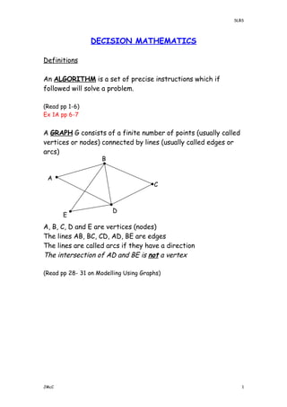
1. SLBS
DECISION MATHEMATICS
Definitions
An ALGORITHM is a set of precise instructions which if
followed will solve a problem.
(Read pp 1-6)
Ex 1A pp 6-7
A GRAPH G consists of a finite number of points (usually called
vertices or nodes) connected by lines (usually called edges or
arcs)
A, B, C, D and E are vertices (nodes)
The lines AB, BC, CD, AD, BE are edges
The lines are called arcs if they have a direction
The intersection of AD and BE is not a vertex
(Read pp 28- 31 on Modelling Using Graphs)
JMcC 1
E
D
C
B
A

2. SLBS
GRAPH THEORY
A PATH is a finite sequence of edges such that the end vertex
of one edge in the sequence is the start vertex of the next.
e.g. ABCDF
A CYCLE (or Circuit) is a closed path, i.e. the end vertex of the
last edge is the start vertex of the first edge.
e.g. ABCDA
A HAMILTONIAN CYCLE is a cycle that passes through every
vertex of the graph once and only once, and returns to its start
vertex. (Not all graphs have such a cycle)
e.g. ABCDFEA
A EULERIAN CYCLE is a cycle that includes every edge of a
graph exactly once. (Not all graphs have such a cycle)
The above graph does not have an Eulerian cycle
The VERTEX SET is the set of all vertices of a graph.
e.g. { A, B, C, D, E, F }
JMcC 2
F
E D
C
BA

3. SLBS
The EDGE SET is the set of all edges of a graph.
e.g. { AB, AD, AE, BC, CD, DE, DF, EF }
a SUBGRAPH of a graph is a subset of the vertices together
with a subset of the edges.
e.g.
Two vertices are CONNECTED if there is a path in G between
them.
A graph is CONNECTED if all pairs of its vertices are
connected.
e.g the above graph is connected but the example below isn’t as
there is no path from A to H
A LOOP is an edge with the same vertex at each end.
e.g.
JMcC 3
D
C
BA
JH
C
BA
B

4. SLBS
A SIMPLE GRAPH is one in which there are no loops and not
more than one edge connecting any pair of vertices.
e.g. the given example is a simple graph (on p 2) but the two
below are not:
there are two edges that connect A and D
there is loop at C
The DEGREE (or VALENCY or ORDER) of a vertex is the
number of edges attached to it.
e.g.
Vertex Degree
A 2
B 4
C 1
D 3
E 2
JMcC 4
D C
BA
C
BA
C and D are odd vertices
A, B and E are even vertices
Note that a loop is regarded as two edges
E
D
C
BA

5. SLBS
A DIGRAPH, which is short for Directed Graph, is a graph
where one or more of the edges has a direction
e.g
Ex 2A pp 34-36
ADJACENY MATRIX
Used for storing in a computer
Each row and each column represent a vertex of the graph and
the numbers in the matrix give the number of edges joining
each pair of vertices.
e.g.
D to D is 2 because you can go in either direction
JMcC
A B C D
A 0 2 1 1
B 2 0 0 1
C 1 0 0 1
D 1 1 1 2
5
E
D
C
B
A
D
C
B
A

6. SLBS
For a Digraph, only include in the matrix the number of edges in
the given direction.
e.g. for earlier example
Ex 2B pp 38-40
JMcC
A B C D E
A 0 1 0 0 1
B 0 0 1 1 1
C 0 1 0 0 0
D 0 0 0 2 0
E 1 1 0 0 0
6

7. SLBS
A TREE is a connected graph with no cycles.
e.g.
The graph below is not a tree as it contains a cycle BCEB
(Read pp 41-42)
A SPANNING TREE of graph G is a subgraph that includes all
the vertices of G and is also a tree.
e.g. a spanning tree (there are others) is shown below the graph
JMcC 7
F
E
DC
B
A
F
E
DC
B
A
E D
C
BA
E D
C
BA

8. SLBS
A COMPLETE GRAPH is one where every vertex is connected
to every other vertex.
If it has n vertices, it is denoted by Kn
K2 K3 K4 K5
Ex 2C Nos 1-3 p 46
A NETWORK is a graph in which each edge or arc is given a
value called its WEIGHT
(see top of p 45)
e.g.
Note: this is not a geometric drawing, the weights do not
represents the lengths of the edges.
JMcC 8
D
CBA 7
5
1016
12

9. SLBS
MINIMAL CONNECTOR PROBLEMS
Problem:
A cable TV company is installing a system of cables to connect
all the towns all the towns in a region. The numbers in the
network show distances in miles.
What is the least amount of cable needed?
We can find a spanning tree (below) but does it use the least
amount of cable? (Solution below uses 76 miles)
JMcC 9
F
E
D
C
B
A
10
8 14
12
15
13
1920
12
F
E
D
C
B
A
10
12
15
1920

10. SLBS
KRUSKAL’S ALGORITHM (1956)
This is an algorithm for finding a minimum spanning tree, or
minimum connector.
This is a spanning tree such that the total length of its edges is
as small as possible.
Kruskal is an example of a GREEDY ALGORITHM
It makes an optimal choice at each stage without reference to
the arcs already chosen as long as no cycles are formed.
JMcC 10
Step 1 Rank the arcs in ascending order of weight
Step 2 Select the arc of least weight and use this to
start the tree
Step 3 Choose the next smallest arc and add this to
the tree UNLESS IT COMPLETES A CYCLE
in which case reject it and proceed to the next
smallest arc
Step 4 Repeat Step 3 until all vertices are included in
the tree

11. SLBS
To solve our TV Cable problem:
Step 1 8 (FE), 10(FD), 12(DB), 12(DE), 13(BC), 14(CE),
15(DC), 19(AB), 20(AD)
Step 2 Select FE
Step 3 a) Select FD
b) DB and DE are of equal length but DE
forms a cycle so DB must be chosen
c) Select BC
d) CE forms a cycle so reject it
e) DC forms a cycle so reject it
f) Select AB
g) AD forms a cycle so reject it
This solution uses 62 miles
In an exam, to show evidence of using the correct algorithm,
you need only list the selected arcs in the order you chose
them
e.g. FE, FD, DB, BC, AB
(Read Examples 1 & 2 pp 52-54)
Ex 3A pp 55-56
JMcC 11
F
E
D
C
B
A
10
8
13
19
12

12. SLBS
Kruskal has two drawbacks:
1) it is necessary to sort the edges in ascending order
first
2) it is necessary at each stage to check for cycles
(difficult for large networks)
Another algorithm which is more easily computerised is:
PRIM’S ALGORITHM (1957)
JMcC 12
Step 1 Choose a starting vertex
Step 2 Connect it to the nearest vertex using the
least arc
Step 3 Connect the nearest vertex not in the tree, to
the tree, using the least arc
(In order to do this, look at all the arcs that
link vertices in the tree with those not in the
tree, choose the smallest and use that to add
the vertex, and its arc, to the tree)
Step 4 Repeat step 3 until all of the vertices are
connected

13. SLBS
To solve our TV Cable problem:
Step 1 Choose vertex A
Step 2 The nearest vertex is B, so add B using arc AB
Step 3 a) Arcs coming from A and B outside the tree
have lengths 20, 12, 13
Nearest vertex is D, so add D using arc BD
b) Arcs coming from A, B and D outside the tree
have lengths 13, 15, 12, 10
Nearest vertex is F, so add F using arc DF
JMcC 13
19
B
A
19
B
A
12D
19
B
A
12
D
F
10

14. SLBS
c) Arcs coming from A, B, D, F outside the tree
have lengths 13, 15, 8
Nearest vertex is E, so add E using arc EF
d) Arcs coming from A, B, D, E, F outside the tree
have lengths 13, 15, 14
Has to be 13, so add C using arc BC
In an exam, to show evidence of using the correct algorithm,
you need only list the selected arcs in the order you chose
them.
AB, BD, DF, FE, BC
JMcC 14
19
B
A
12
D
F
10
8
E
19
B
A
12
D
F
10
8
E C
13

15. SLBS
This gives the same solution as Kruskal as there is only one minimum
spanning tree for this network. However, the order in which the arcs is
chosen is different and this is the evidence that you have used the
correct algorithm to solve the problem.
You may get a different solution if there is more than one minimal
spanning tree for a network.
Problems with Kruskal
Candidates get cold feet when they see the tree being built up out of
splinters and use a highbred of Prim and Kruskal, choosing the least
couple of arcs initially and then using Prim’s algorithm thereafter.
Candidates do not spot arcs that complete cycles and do not exclude
them.
Candidates do not make the order of arc selection clear for the
examiners.
Problems with Prim
Candidates only look at the arcs incident on the last connected vertex -
creating a chain of arcs.
Candidates do not make the order of arc selection clear for the
examiners.
Candidates either stop too soon or get rather carried away and don’t
stop.
You will be told which vertex to start with.
Prim is better than Kruskal as it can be computerised easily in matrix
form.
Kruskal’s algorithm adds one edge at a time to a subgraph, whereas Prim’s
algorithm adds one vertex at a time.
Remember for both algorithms:
JMcC 15

16. SLBS
the number of arcs in a final minimum spanning tree
should be one less than the number of vertices
(think fence posts and panels)
JMcC 16

17. SLBS
MATRIX FORM OF PRIM’S ALGORITHM
A network may be described using a DISTANCE MATRIX
For our TV Cable problem, the distance matrix is:
A B C D E F
A - 19 - 20 - -
B 19 - 13 12 - -
C - 13 - 15 14 -
D 20 12 15 - 12 10
E - - 14 12 - 8
F - - - 10 8 -
Note the symmetry of the matrix; the first row is the same as
the first column, the second row is the same as the second
column, etc.
JMcC 17
Step 1 Choose a starting vertex and delete all
elements in that vertex’s row and arrow its
column
Step 2 Neglecting all deleted terms, scan all arrowed
columns for the lowest available element and
circle that element
Step 3 Delete the circled element’s row and arrow its
column
Step 4 Repeat steps 2 and 3 until all rows deleted
Step 5 The spanning tree is formed by the circled
arcs

18. SLBS
1 2 6 3 5 4
A B C D E F
A - 19 - 20 - -
B 19 - 13 12 - -
C - 13 - 15 14 -
D 20 12 15 - 12 10
E - - 14 12 - 8
F - - - 10 8 -
Comparing the matrix algorithm with the network algorithm, it
is seen that the choice and order of selection of the arcs is
identical.
In an exam, the final matrix can look as if a bomb hit it!
(difficult to award marks in these circumstances)
So, number the columns in the order you arrow them and write
down the arcs in the order they are selected.
AB, BD, DF, FE, BC
(Read pp 58-60)
Ex 3B pp 60-63
JMcC 18

19. SLBS
DIJKSTRA’S ALGORITHM (1959)
This is for finding the shortest path in a network.
This is another example of a greedy algorithm.
(Read pp 63-64)
Use the following type of box:
JMcC
Vertex letter Order of
selection
Final values
Working values
19
Step 1 Label the start vertex S with a permanent
label of 0
Step 2 Put a temporary label on each vertex that can be
reached directly from the vertex that has just
received a permanent label. The temporary label must
be equal to the sum of the permanent label and the
weight of the arc linking it directly to the vertex. If
there is already a temporary label at the vertex, it is only
replaced if the new sum is smaller.
Step 3 Select the minimum temporary label and make it
permanent.
Step 4 Repeat steps 2 and 3 until the destination vertex T
receives its permanent label.
Step 5 Trace back from T to S including an arc AB
whenever the permanent label of B − permanent
label of A = the weight of AB, given that B already
lies on the path

20. SLBS
Example
Find the shortest path from A to F
What you will be given in the exam is a diagram like this:
JMcC 20
F
E
D
C
B
A
8
3
4
9
5
7
5
9
5
7
9
9
3
5
8
4
F
E
D
C
B
A

21. SLBS
Solution: (numbers in the “Working Values” box can only be
replaced by a smaller number)
Working backwards from F
16 − 3 = 13 so DF
13 − 9 = 4 so CD ← Show this!
4 − 4 = 0 so AC
So tracing back gives F → D → C → A
Hence the shortest path from A to F is: ACDF
Length of shortest path = 16
Note:
1) Don’t cross values out (examiners need to see them)
2) Do not forget to give temporary labels to all deserving
vertices
3) The permanent label must be awarded to the smallest
temporary label
4) Explain your method by showing the tracing back
(Read pp 65-69)
Ex 3C pp 69-71
JMcC 21
5
7
9
9
3
5
8
4
F
E
D
C
B
A
16
3 7
7
1 0
2
4
4
5
13
13
4
13 12
12
6
17
16

22. SLBS
A BIPARTITE GRAPH consists of two sets of vertices, X and
Y. The edges only join vertices in X to vertices in Y, not
vertices within a set.
e.g.
A COMPLETE BIPARTITE GRAPH is where every vertex in X is
joined to every vertex in Y
e.g.
This graph is known as K3,2
Two graphs are ISOMORPHIC if they have the same number of
vertices and the degrees of corresponding vertices are the
same
e.g.
JMcC 22
R
Q
P
D
C
B
A
Q
P
C
B
A
Q
P
C
B
A A
B
C
P
Q

23. SLBS
A PLANAR GRAPH is one that can be drawn in a plane such that
there are no edges crossing. (No paths cross!)
Microchips are planar networks.
This graph is obviously planar ↑
This graph ↑ does not seem to be planar, but if we redraw it as
follows:
It can be drawn with no edges crossing, therefore it is planar.
How can we decide if a graph is planar or not?
JMcC 23

24. SLBS
A PLANARITY ALGORITHM
This can only be applied to graphs that have a Hamiltonian cycle
(a cycle that passes through every vertex of the graph once
and only once, and returns to its start vertex)
JMcC 24
Step 1 Identify a Hamiltonian cycle in the graph
Step 2 Redraw the graph so that the Hamiltonian
cycle forms a regular polygon and all edges
are drawn as straight lines in the polygon
Step 3 Choose any edge AB and decide this will stay
inside the polygon
Step 4 Consider any edges that cross AB
(a) if it is possible to move all these outside
without producing crossings, go to step 5
(b) if it is not possible then the graph is non
planar
Step 5 Consider each remaining crossing inside and
see if any edge may be moved outside to
remove it, without creating a crossing inside
Step 6 Stop when all crossings inside have been
considered
(a) if there are no crossings inside or outside
then the graph is planar
(b) if there is a crossing inside that cannot be
removed then the graph is non-planar

25. SLBS
Example
1) Choose Hamiltonian cycle ABCDEFGHA (already a
polygon)
2) Choose any arc in original graph not in the cycle (say AE)
and list other arcs in the cycle which cross this chosen
arc (BG and BH)
This means that the chosen arc and the arcs it crosses
must be separated by the polygon
3) Formulate a bipartite list by placing the first arc on one
side (IN) and the list of the other arcs on the other side
(OUT). Arcs which cross are incompatible.
IN OUT
AE BG
BH
JMcC 25
H
G
F
E
D
C
B
A
H
G
F
E
D
C
B
A

26. SLBS
4) Now choose one of the arcs on the OUT side, and list any
arcs which are incompatible with it. Put these arcs as
vertices on the IN side.
(Choose BG say. The new arcs which cross it are AC, AD,
EH and FH. These all now appear on the IN side)
IN OUT
AE BG
AC BH
AD
EH
FH
5) Select each new OUT arc in turn and list any new
incompatible arcs on IN side.
(Moving onto BH, there are no new arcs to add to the IN
side and there are no more arcs on the OUT side to
consider)
JMcC 26
H
G
F
E
D
C
B
A

27. SLBS
6) Select each IN arc in turn and list any new incompatible
arcs on the OUT side.
(Choosing AC we add BE to the OUT side, BG & BH are
already there)
IN OUT
AE BG
AC BH
AD BE
EH
FH
(choosing AD we add EC to the OUT side, BE, BG & BH are
already there)
IN OUT
AE BG
AC BH
AD BE
EH EC
FH
JMcC 27
H
G
F
E
D
C
B
A

28. SLBS
(choosing EH we have nothing to add, choosing FH we add EG to
the OUT side)
IN OUT
AE BG
AC BH
AD BE
EH EC
FH EG
JMcC 28
H
G
F
E
D
C
B
A
H
G
F
E
D
C
B
A

29. SLBS
7) Continue until all arcs have been added
8) The planar graph can now be drawn. All the arcs on the
IN side of the bipartite list are drawn “inside” the
Hamiltonian cycle and all the arcs on the OUT side
“outside” the cycle.
A
B
C
D
E
F
G
H
(Read pp 73-75)
Ex 3D pp 75-76
JMcC 29

30. SLBS
THE ROUTE INSPECTION PROBLEM
A TRAVERSABLE graph is one that can be drawn without
removing your pen from the paper and without going over the
same edge twice.
The sum of degrees of the vertices is always twice the number
of edges (Handshaking theorem) ∑ deg v = 2e
Since the sum of the degrees of the vertices is always even, it
follows that there will always be an even number of odd
vertices. (Handshaking lemma)
If we start at vertex X and finish at vertex Y.
Assume X and Y are different vertices
One edge is used when we leave X and each time we return to X
we must arrive and leave by new edges.
Hence the vertex X must have an odd valency. It’s called an odd
vertex.
Similarly Y must be an odd vertex.
All remaining vertices must be even, since every time we pass
through an intermediate vertex (not X or Y) we use two edges.
JMcC
A route starting and finishing at different vertices X and Y is
only possible if X and Y are odd vertices and all the other
vertices are even. (Then the graph is called semi-Eulerian)
30
leave
return
X

31. SLBS
Vertices A and D are odd
Vertices B, C and E are even
It is semi-Eulerian.
It can be drawn by starting at A and finishing at D by using the
route
ABCDEAD
If X = Y
X must be even, therefore:
All vertices have degree 2 and are even. It is Eulerian. It can
be drawn by starting and finishing at A using the route AECBDA
JMcC
If the start and finish vertices are the same, all vertices must
be even.
The graph is called Eulerian.
31
E
D
C
BA
Start
Finish
X
E
D
C
BA

32. SLBS
THE SEVEN BRIDGES OF KONIGSBERG
The town of Konigsberg in Eastern Prussia (later renamed
Kalingrad) was built on the banks of the River Pregel, with
islands that were linked to each other and the river banks by
seven bridges.
A
B
C
D
The citizens of the town tried for many years to find a route
for a walk which would cross each bridge only once and allow
them to end their walk where they had started.
Leonhard Euler (1707-1783) translated this practical problem
into a graph theory problem.
Representing the areas A, B, C and D as vertices and the 7
bridges as arcs, we obtain the following graph
All the vertices are odd. Graph is not Eulerian.
Therefore the graph is not traversable and there is no solution!
Ex 4A pp 90-91
JMcC 32
D
C
B
A

33. SLBS
THE CHINESE POSTMAN PROBLEM
[Mei-Ku Kwan in 1962]
A postman wishes to deliver his letters by covering the
shortest possible distance and return to his starting point.
If the graph is Eulerian it is traversable.
If it has some odd vertices then some arcs will have to be
repeated. These repeats will be such that when added to the
graph it will make the odd vertices even! This new graph is now
Eulerian and therefore traversable. We need to find the
repeats that make the total distance of these repeats as small
as possible.
Note:
1) Make sure you consider all possible pairings
2) Make it clear which pairs you are using
JMcC 33
Step 1 Identify all the odd vertices
Step 2 Form all possible pairings of odd vertices
Step 3 For each pairing find the arcs that make the total
distance of repeats as small as possible
Step 4 Choose the pairing with the smallest sum and add
this to the graph
Step 5 Find a route that works and add the smallest sum
found in Step 4 to the sum of all the weights in the
original graph to find the length of the required
route.

34. SLBS
3) Remember to state the route at the end!
JMcC 34

35. SLBS
Example
A postman starts at the depot T and has to deliver mail along
all the streets shown in the network below. Find a route that
means he travels the shortest possible distance.
All distances are in km.
JMcC 35
T
HG
F
E
D
CB
A
0.8
1.7
1.01.0
2.0 0.75
0.2
0.4 0.6
0.5 1.5
1.7
0.6
0.9
1.6
0.9
0.3

36. SLBS
Solution
Step 1 Odd vertices are B(3), G(3), H(3), T(3)
Steps 2 and 3
Pairing Shortest Route Distance
BG and HT
BH and GT
BT and GH
BEG + HECT
BEH + GECT
BCT + GH
1.7 + 1.8 = 3.5
1.5 + 2.0 = 3.5
0.8 + 0.9 = 1.7
Step 4 The pairing with the smallest sum is BT and GH
A possible route is TABEAGHEGHFDFECDTCBCT
Total weight of original graph = 17.25
Smallest sum of repeated edges = 1.7
Length of traversable route = 17.25 + 1.7 = 18.95 km
(Read Examples 1, 2 and 3 pp 92-95 + Special Case on p 96)
Ex 4B pp 96-99
JMcC 36
T
HG
F
E
D
CB
A
0.8
1.7
1.01.0
2.0 0.75
0.2
0.4 0.6
0.5 1.5
1.7
0.6
0.9
1.6
0.9
0.3