this is an example......

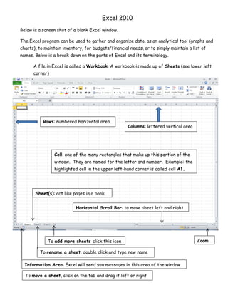
1. Excel 2010
Below is a screen shot of a blank Excel window.
The Excel program can be used to gather and organize data, as an analytical tool (graphs and
charts), to maintain inventory, for budgets/financial needs, or to simply maintain a list of
names. Below is a break down on the parts of Excel and its terminology.
A file in Excel is called a Workbook. A workbook is made up of Sheets (see lower left
corner)
Rows: numbered horizontal area
Columns: lettered vertical area
Cell: one of the many rectangles that make up this portion of the
window. They are named for the letter and number. Example: the
highlighted cell in the upper left-hand corner is called cell A1.
Sheet(s): act like pages in a book
Horizontal Scroll Bar: to move sheet left and right
To add more sheets click this icon Zoom
To rename a sheet, double click and type new name
Information Area: Excel will send you messages in this area of the window
To move a sheet, click on the tab and drag it left or right

2. Tabs
Box Launcher: click on this
icon to see more less used
Ribbon: grey area commands
Command: icons that allow you to perform
Groups – related
tasks or make changes in the workbook
commands
Contextual Tab: This tab will appear if
an object is inserted and selected in
your sheet (page). It allows you to edit
the inserted image or object.
Formula Bar: Shows you what is exactly in each cell.
Name Bar: Shows you which cell you are in (or is highlighted)
Fill Series: Type in your first (sometimes first and
second) value(s) in a cell. Then select the cell(s) and
click on the little square in the lower right corner of
the cell. Drag down or to the right to fill cells.
Height and Width: Two ways…
1.) Right click the cell and select column width or Row
Height. Adjust as you wish.
2.) Double click on the line between the column letter
you want to adjust and the next column letter. For
example. To adjust column D, click on the line
between D and E. To adjust row 3, click and drag on
the between the 3 and the 4.
To delete a column or row: Right click on the letter or number you
want to remove. Right click and then select delete.
Never skip rows or columns! Adjust spacing my making the cells larger or smaller

3. To Create a Graph using your Excel Data
To create a graph you must remember what needs to be included to properly display your
data in a way that can be read and analyzed.
Remember to think about TAILS and DRY MIX
T- Title D- Dependent Variable M- Manipulated (Ind) Variable
A- Axis R- Responding variable I-Independent variable
I- Intervals Y- Y Axis X- X Axis
L- Labels
S- Scale
Column A is for data you want on the x-axis
This is your Independent Variable
Column B is for data you want on your y-axis
This is your Dependent Variable
Include a brief but fully descriptive heading at the top of each column explaining the
data.
Include units of measurement. As long as you include them in the column heading you
do not have to list them after each data value. In fact you do not want to include
them in an Excel data table as it will show up on your graph.
Convert all data in the “Column A” to text. First, highlight the cells your data will fill.
Select the Home Tab. Select Text in the Number Group. Then input your data. Be
sure the blue triangle shows up in the upper left corner of each cell you add data to.

4. Step 1
Click on A1, holding down the left mouse key and
select your entire data table (click and drag)
Step 2
Click the Insert Tab. Select the Chart you want to
use (for a line or bar graph). This example will be for
a line graph
Step 3
When you select your graph it will appear in the
middle of your data sheet. Click on the edge of the
entire graph to select it and click on the command
Move Chart Location then click on “New Sheet”. Later
remember to rename that new sheet “Graph”.
Step 4
In your new sheet, select the graph.
Then click on Design under the Chart
Contextual Tab. Click the Arrow on the
right side of the Chart Layouts and
choose the graph example that best fits
your needs.

5. Step 5
You will see the graph now has additional
information and needs editing.
Click on and delete the Legend or Key, you
don’t need one for this graph. (You will
need a key on some graphs).
Step 6
You will see the graph now has additional information and needs editing.
Edit the graph to fulfill the requirements of your assignment. This is when you can
adjust your font color/size, graph colors, etc.
Step 7 Print Preview icon
Printing
Use the Print Preview command to view and edit your graph before printing. Set the page
orientation to Landscape in Page Setup. On the Header/Footer tab, use Custom Footer to
enter your full name, the project title and current date.