abaqus,Workshop

1. Workshop 1
Linear Static Analysis of a Cantilever Beam
Introduction
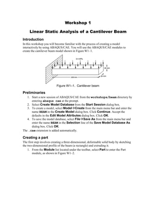
In this workshop you will become familiar with the process of creating a model
interactively by using ABAQUS/CAE. You will use the ABAQUS/CAE modules to
create the cantilever beam model shown in Figure W1–1.
Figure W1–1. Cantilever beam
Preliminaries
1. Start a new session of ABAQUS/CAE from the workshops/beam directory by
entering abaqus cae at the prompt.
2. Select Create Model Database from the Start Session dialog box.
3. To create a model, select ModelCreate from the main menu bar and enter the
name BEAM in the Create Model dialog box. Click Continue. Accept the
defaults in the Edit Model Attributes dialog box. Click OK.
4. To save the model database, select FileSave As from the main menu bar and
enter the name BEAM in the Selection line of the Save Model Database As
dialog box. Click OK.
The .cae extension is added automatically.
Creating a part
The first step involves creating a three-dimensional, deformable solid body by sketching
the two-dimensional profile of the beam (a rectangle) and extruding it.
1. From the Module list located under the toolbar, select Part to enter the Part
module, as shown in Figure W1–2.

2. Figure W1–2. Module list
5. From the main menu bar, select PartCreate to create a new part.
The Create Part dialog box appears.
6. Name the part Beam. Accept the default settings of a three-dimensional,
deformable body and a solid, extruded base feature in the Create Part dialog
box. In the Approximate size text field, type 300.
7. Click Continue to exit the Create Part dialog box.
ABAQUS/CAE displays text in the prompt area near the bottom of the window to guide
you through the procedure, as shown in Figure W1–3. Click the cancel button to cancel
the current task; click the backup button to cancel the current step in the task and return to
the previous step.
Figure W1–3. Prompt area
The Sketcher toolbox appears in the left side of the main window, and the Sketcher grid
appears in the viewport.
To sketch the profile of the cantilever beam, you need to draw a rectangle. To select the
rectangle drawing tool, do the following:
A. Note the small black triangles at the base of some of the toolbox icons. These
triangles indicate the presence of hidden icons that can be revealed. With
mouse button 1, click and hold the Create Lines tool in the upper-right
corner of the Sketcher toolbox. Additional icons appear, as shown in
Figure W1–4.
W.2

3. Figure W1–4. Selecting a tool
B. Without releasing mouse button 1, drag the cursor along the set of icons that
appear. Release the mouse button when you reach the rectangle tool to select
that tool.
The rectangle drawing tool appears in the Sketcher toolbox with a pink background,
indicating that you selected it. ABAQUS/CAE displays prompts in the prompt area to
guide you through the procedure. In the viewport, sketch the rectangle by doing the
following:
C. Notice that as you move the cursor around the viewport, ABAQUS/CAE
displays the cursor’s X- and Y-coordinates in the upper-left corner.
D. Click one corner of the rectangle at coordinates (100, 10).
E. Move the cursor to the opposite corner (100, 10) so that the rectangle is
20 grid squares long and 2 grid squares high, as shown in Figure W1–5.
Figure W1–5. Rectangle drawn with sketcher
F. Click mouse button 1 to create the rectangle.
G. Click mouse button 2 anywhere in the viewport to finish using the rectangle
tool. (Mouse button 2 is the middle mouse button on a 3-button mouse; on a 2-
button mouse, press both mouse buttons simultaneously.)
H. Click Done in the prompt area to exit the sketcher.
I. Enter an extrusion depth of 25 in the Edit Base Extrusion dialog box, and
click OK.
ABAQUS/CAE displays an isometric view of the new part, as shown in Figure W1–6.
W.3

4. Figure W1–6. Extruded part
Creating a material definition
You will now create a single linear elastic material with a Young’s modulus of
209103
MPa and Poisson’s ratio of 0.3.
To define a material:
1. In the Module list located under the toolbar, select Property to enter the
Property module.
8. From the main menu bar, select MaterialCreate to create a new material.
9. Name the material Steel, and click Continue.
Notice the various options available in the Edit Material dialog box.
Figure W1–7. Pull–down menu
10. From the material editor’s menu bar, select MechanicalElasticityElastic,
as shown in Figure W1–7.
ABAQUS/CAE displays the Elastic data form.
11. Enter a value of 209.E3 for Young’s modulus and a value of 0.3 for Poisson’s
ratio in the respective fields, as shown in Figure W1–8. Use [Tab] to move
between cells, or use the mouse to select a cell for data entry.
W.4

5. Figure W1–8. Material editor
12. Click OK to exit the material editor.
Defining and assigning section properties
To define the homogeneous solid section:
1. From the main menu bar, select SectionCreate.
13. In the Create Section dialog box:
A. Name the section BeamSection.
J. In the Category list, accept Solid as the default category selection.
K. In the Type list, accept Homogeneous as the default type selection.
L. Click Continue.
The solid section editor appears.
14. In the Edit Section dialog box:
A. Accept the default selection of Steel for the Material associated with the
section.
M. Accept the default value of 1 for Plane stress/strain thickness.
N. Click OK.
To assign the section definition to the cantilever beam:
1. From the main menu bar, select AssignSection.
ABAQUS/CAE displays prompts in the prompt area to guide you through the procedure.
15. Click anywhere on the beam to select the region to which the section will be
assigned.
ABAQUS/CAE highlights the entire beam.
16. Click mouse button 2 in the viewport or click Done in the prompt area to accept
the selected geometry.
The Assign Section dialog box appears containing a list of existing section definitions.
17. Accept the default selection of BeamSection as the section definition, and click
OK.
ABAQUS/CAE assigns the solid section definition to the beam and closes the Assign
Section dialog box.
Assembling the model
To assemble the model:
1. In the Module list located under the toolbar, select Assembly to enter the
Assembly module.
W.5

6. 18. From the main menu bar, select InstanceCreate.
19. In the Create Instance dialog box, select Beam and click OK.
Configuring the analysis
To create a general, static analysis step:
1. In the Module list located under the toolbar, select Step to enter the Step
module.
20. From the main menu bar, select StepCreate to create a step.
21. Name the step BeamLoad.
22. From the list of available general procedures in the Create Step dialog box,
select Static, General if it is not already selected and click Continue.
23. In the Description field of the Basic tabbed page, type Load the top of
the beam.
24. Click the Incrementation tab, and delete the value of 1 that appears in the
Initial text field. Type a value of 0.1 for the initial increment size.
25. Click the Other tab to see its contents; you can accept the default values provided
for the step.
26. Click OK to create the step and to exit the step editor.
Applying a boundary condition and a load to the model
To apply boundary conditions to one end of the cantilever beam:
1. In the Module list located under the toolbar, select Load to enter the
Load module.
27. From the main menu bar, select BCCreate.
28. In the Create Boundary Condition dialog box:
A. Name the boundary condition Fixed.
O. Select Initial as the step in which the boundary condition will be activated.
P. In the Category list, accept Mechanical as the default category selection.
Q. In the Types for Selected Step list, select Displacement/Rotation as
the type and click Continue.
ABAQUS/CAE displays prompts in the prompt area to guide you through the procedure.
29. The face at the end of the cantilever beam will be fixed. Click the Show/Hide
Selection Options icon in the prompt area to open the Options dialog
box. Deselect Select entity closest to the screen in the Options dialog box
so that you can pick the desired face, as shown in Figure W1–9.
W.6

7. Figure W1–9. Correct face selected
ABAQUS/CAE may not be able to determine what you selected; in that case, it will select
the face closest to you and display buttons in the prompt area that allow you to choose the
required face. To cycle through the valid selections, do the following:
A. From the prompt area, click Next or Previous until the desired face is
selected.
R. Click OK to accept the current selection.
30. Click mouse button 2 in the viewport or click Done in the prompt area to accept
the selected geometry.
The Edit Boundary Condition dialog box appears. When you are defining a boundary
condition in the initial step, all six degrees of freedom are unconstrained by default.
31. In the Edit Boundary Condition dialog box:
A. Toggle on U1, U2, and U3, since only the translational degrees of freedom
need to be constrained (the beam will be meshed with solid elements later).
S. Click OK to create the boundary condition definition and to exit the editor.
ABAQUS/CAE displays arrows at each corner and midpoint on the selected face to
indicate the constrained degrees of freedom.
To apply a load to the top of the cantilever beam:
1. From the main menu bar, select LoadCreate.
The Create Load dialog box appears.
32. In the Create Load dialog box:
A. Name the load Pressure.
T. Select BeamLoad as the step in which the load will be applied.
U. In the Category list, accept Mechanical as the default category selection.
V. In the Types for Selected Step list, select Pressure.
W. Click Continue.
ABAQUS/CAE displays prompts in the prompt area to guide you through the procedure.
33. In the viewport, select the top face of the beam as the surface to which the load
will be applied. The desired face is shown by the gridded face in Figure W1–10.
W.7

8. Figure W1–10. Fixed boundary conditions
34. Click mouse button 2 in the viewport or click Done in the prompt area to indicate
that you have finished selecting regions.
35. In the Edit Load dialog box:
A. Enter a magnitude of 0.5 for the load.
X. Accept the default Amplitude selection (Ramp) and the default
Distribution (Uniform).
Y. Click OK to create the load definition and to exit the editor.
ABAQUS/CAE displays downward pointing arrows along the top face of the beam to
indicate the load applied in the negative 2-direction.
Meshing the model
You use the Mesh module to generate the finite element mesh. You can choose the
meshing technique that ABAQUS/CAE will use to create the mesh, the element shape,
and the element type. ABAQUS/CAE uses a number of different meshing techniques. The
default meshing technique assigned to the model is indicated by the color of the model
when you enter the Mesh module; if ABAQUS/CAE displays the model in orange, it
cannot be meshed without assistance from the user.
To assign the mesh controls:
1. In the Module list located under the toolbar, select Mesh to enter the Mesh
module.
36. From the main menu bar, select MeshControls.
37. In the Mesh Controls dialog box, accept Hex as the default Element Shape
selection.
38. Accept Structured as the default Technique selection.
39. Click OK to assign the mesh controls and to close the dialog box.
To assign an ABAQUS element type:
1. From the main menu bar, select MeshElement Type.
40. In the Element Type dialog box, accept the following default selections that
control the elements that are available for selection:
W.8

9. · Standard is the default Element Library selection.
· Linear is the default Geometric Order.
· 3D Stress is the default Family of elements.
41. In the lower portion of the dialog box, examine the element shape options. A brief
description of the default element selection is available at the bottom of each
tabbed page.
42. In the Hex page, select Incompatible modes.
A description of the element type C3D8I appears at the bottom of the dialog box.
ABAQUS/CAE will now mesh the part with C3D8I elements.
43. Click OK to assign the element type and to close the dialog box.
To mesh the model:
1. From the main menu bar, select SeedInstance to seed the part instance.
The prompt area displays the default element size that ABAQUS/CAE will use to seed
the part instance. This default element size is based on the size of the part instance.
44. In the prompt area, enter a global element size of 10 and press [Enter] or click
mouse button 2 in the viewport.
45. ABAQUS/CAE applies the seeds to the part, as shown in Figure W1–11.
Figure W1–11. Seeded part instance
46. From the main menu bar, select MeshInstance to mesh the part.
47. Click Yes in the prompt area or click mouse button 2 in the viewport to confirm
that you want to mesh the part instance.
48. ABAQUS/CAE meshes the part instance and displays the resulting mesh, as
shown in Figure W1–12.
W.9

10. Figure W1–12. Part instance showing the resulting mesh
Creating and submitting an analysis job
To create and submit an analysis job:
1. In the Module list located under the toolbar, select Job to enter the Job module.
49. From the main menu bar, select JobCreate to create a job.
The Create Job dialog box appears.
50. Name the job Deform.
51. From the list of available models select BEAM.
52. Click Continue to create the job.
53. In the Description field of the Edit Job dialog box, enter Workshop 1.
54. Click the tabs to see the contents of each folder of the job editor and to review the
default settings. Click OK to accept the default job settings.
55. Select JobManager to start the Job Manager.
56. From the buttons on the right edge of the Job Manager, click Submit to submit
your job for analysis. The status field will show Running.
57. When the job completes successfully, the status field will change to Completed.
You are now ready to view the results of the analysis in the Visualization module.
Viewing the analysis results
1. Click Results in the Job module’s Job Manager to enter the Visualization
module.
ABAQUS/CAE opens the output database created by the job (Deform.odb) and
displays a fast plot of the model, as shown in Figure W1–13.
W.10

11. Figure W1–13. Fast plot of the model
58. From the main menu bar, select PlotUndeformed Shape to view the
undeformed model shape plot.
59. From the main menu bar, select PlotDeformed Shape to view a deformed
model shape plot, as shown in Figure W1–14.
Figure W1–14. Deformed model shape
You may need to use the Auto-Fit View tool to rescale the figure in the viewport.
60. From the main menu bar, select PlotContours to view a contour plot of the
von Mises stress, as shown in Figure W1–15.
W.11

12. Figure W1–15. Mises stress contour plot
61. From the main menu bar, select FileSave to save your model in a model
database file. Close the ABAQUS/CAE session by selecting FileExit from the
main menu bar.
62. Rename the abaqus.rpy replay file BEAM.rpy. Start a new ABAQUS/CAE
session, and execute the replay file using the command
abaqus cae replay=BEAM.rpy
Commands issued during the previous ABAQUS/CAE session are executed automatically
through the replay Python script. Close the ABAQUS/CAE session by selecting
FileExit from the main menu bar.
63. Start a new ABAQUS/CAE session, and rebuild the BEAM.cae model database
using the command
abaqus cae recover=BEAM.jnl
Only the commands necessary to rebuild the model database BEAM.cae are executed.
W.12