1. FACTS, FIGURES AND STATISTICS
“Lies, damn lies, and statistics” Mark Twain
“But some damned lies are the truth” PDW
“When in doubt tell the truth” also Mark Twain
Statistics is the systematic selection, presentation and assessment of numerically based data. When
information available is less than complete statistics can minimize, but never completely exclude, the
risk of erroneous conclusions. Skepticism is important. Statistics has practical limitations: the chances
of your existing and reading this book are almost zero, but has turned out to be reality: almost
incredibly each and every one of your ancestors (starting with unicellular organisms) was fertile!
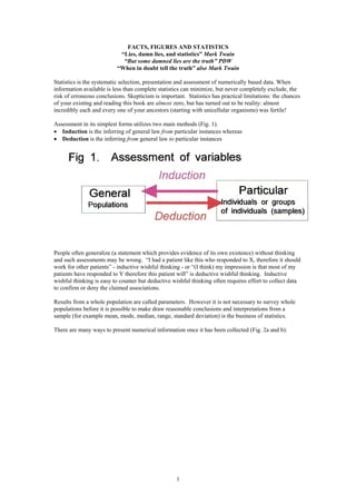
Assessment in its simplest forms utilizes two main methods (Fig. 1).
• Induction is the inferring of general law from particular instances whereas
• Deduction is the inferring from general law to particular instances
People often generalize (a statement which provides evidence of its own existence) without thinking
and such assessments may be wrong. “I had a patient like this who responded to X, therefore it should
work for other patients” - inductive wishful thinking - or “(I think) my impression is that most of my
patients have responded to Y therefore this patient will” is deductive wishful thinking. Inductive
wishful thinking is easy to counter but deductive wishful thinking often requires effort to collect data
to confirm or deny the claimed associations.
Results from a whole population are called parameters. However it is not necessary to survey whole
populations before it is possible to make draw reasonable conclusions and interpretations from a
sample (for example mean, mode, median, range, standard deviation) is the business of statistics.
There are many ways to present numerical information once it has been collected (Fig. 2a and b).
1
3. Samples
Results obtained from samples can never be certain. All we can have is probability and levels of
confidence.
Obviously samples should be representative of the population about which a generalization is sought.
Vaguely selected samples, especially those defined in retrospect - “the patients I have seen” - are
unlikely to be representative. Samples are more likely to be representative if a researcher selects his
sample randomly from the population under study. Randomly does not mean haphazard - haphazard
often means that the bias of selection is unrecognized and unacknowledged. Lists of random numbers
are available to assist this process but if the same sequence of random numbers is used repeatedly then
bias might be introduced.
Random allocation of an intervention should ensure that the intervention and non-intervention groups
are similar because three should be no allocation bias. Observer bias should be abolished by having a
double blind trial in which the observer does not, and cannot, suspect whether a patient has or has not
received the intervention and then a difference in results must be attributable, directly or indirectly, to
the intervention.
There is more chance of a sample being representative if:
• A large sample of the population under study is used
• There is an automatic “mechanical” selection process
• Stratification is used if necessary (the population studied might comprise hidden subgroups,
membership of which might influence the outcome). Subgroups of the population might give
different replies because they are members of a subgroup and this, if unrecognized, may invalidate
results (Fig. 3). For example failure to stratify a sample according to whether those sampled were
male or female might lead to inappropriate generalizations for behavior of the whole population.
3
4. Samples are surveyed for the presence of the characteristic(s) under study - the variables (Fig. 3).
There are two types of variable. Numerical variables (each variable has an intrinsic numerical value,
weight for example) or category variable (each variable either is or is not a something, male or female
for example).
Definitions
The mean, colloquially “the average,” is the most commonly used statistic in everyday conversation. It
is an intuitively reassuring, although possibly fallible, measure of what is “normal.” The mean is the
total of numerical variables divided by the number of such variables. Means tend to remain stable over
successive samples
The median is the middle observation in a series (if there is an even number of observations the median
is taken to be halfway between the two middle observations)
The mode is the value of the most frequent observation (usually used in assessment of category
variables)
The range is the numerical difference between the numerical value of the highest and lowest
observation
4
5. The mean tells us little of the distribution of the numerical results (the means of 2,2,2,2,2,2 and
8,8,8,8,8,8 is 5 as is the mean of 4,4,4,4,4,4 and 6,6,6,6,6). A measure of scatter, “dispersion,” or
variability of the numerical variables is required. One commonly used measure is the Standard
Deviation (Fig. 4). A useful gauge of scatter would be the average distance from the average.
However to confuse matters statisticians count differences above the mean as positive and below as
negative and thus if the differences each side of the mean are added the result is zero. To avoid this
difficulty statisticians square each difference from the mean (a negative squared then becomes
positive) and statisticians then take the square root of the sum of the squares which is designated as the
Standard Deviation). This is not the same as average distance from the average.
COMMON MISAPPREHENSIONS
The mean “average” = the median. Consider 1,2,3,4,7,8,10. The mean is 35/7 =5 yet the
median is 4 (this constitutes a skewed distribution)
The mode = the mean “average” Consider 1,222,3,7,11. The mode is 2 and the mean is 4
It is meaningful to calculate means or median for category variables. Is the mean member of
the population 56 percent female?
Observations outwith two standard deviations either side of the mean (equivalent to 5 percent of
observations) are unusual and are often regarded, somewhat arbitrarily, as abnormal and worthy of
comment and/or investigation.
The distribution of numerical variables can be symmetrical or skewed (Fig. 6). Most but not all
biological curves of distribution are of normal distribution (being symmetrical and bell shaped) with
the mean being central. With more observations the curves of distribution become smoother. Any one
value can be rated as “so many standard deviations from the mean.” The distance between the mean
and the point of inflection “bending back” of a normal curve is one standard deviation from the mean
(Fig. 4). Sixty-eight percent (roughly two thirds) of observations in a normal curve of distribution lie
within the two standard deviations straddling the mean.
5
6. Standard deviations above (or below) the mean can be used to compare single results from two sets of
observations “Jim’s anatomy exam result was 1.25 standard deviations above the mean whereas in
physiology he scored 1.1 standard deviations below the mean. This tells us that Jim was better than his
peers at anatomy and worse in physiology even though he may have scored higher marks in physiology
than anatomy (as would occur if most candidates had high marks in physiology but only a few had
high marks in anatomy”).
When there are two or more separate peaks well away from the mean the standard deviation (which
after all is a single numerical value) alone will not reveal the two-peaked shape of the curve. If there
are two or more peaks in curves obtained from biological observations suspect two subgroups (Fig. 5)
in the sample or a quirk in data collection (for example measuring the distance of the right and left eye
from the right ear would automatically give rise to two peaks).
Even if the curve of distribution of the population is not normal (is skewed) the means of several
different samples from the same population can be obtained and the curve of distribution of these
means will be a normal curve and the standard deviation of the samples from their mean can be
obtained. Then 68 percent (one standard deviation each side of the mean) of the samples will lie
within one standard deviation each side of the samples mean. This is known as the standard error. The
importance of this is that a sample which yield a mean outwith this value become more likely to be
unreliable. The extent of a standard error is mostly related to the proportion of the population covered
by the samples, variability of the population, or size of the samples
The smaller the standard error of a particular sample, the more likely it is that a particular sample mean
is close to the population mean. There is a 68 percent probability that a particular sample mean plus or
minus one standard error contains the population mean (also a 32 percent chance that it does not).
This is the 68 percent confidence interval. A confidence interval of 95 percent covers (approximately)
plus or minus two standard errors and is the same as saying that there is less than one chance in 20 that
the results are caused by chance. A 99 percent confidence interval covers (approximately) plus or
minus two and half standard errors and is the same as saying that there is less than one chance in a
hundred that the results are caused by chance. The larger the difference in standard error between two
samples then the more it is likely that the difference between the two samples is significant.
6
7. When comparing two sets of results the null hypothesis (that there is no difference between two sets of
results) has to be proved wrong. There are two types of error:
• Type 1 error is accepting a difference as significant when it isn’t (falsely rejecting the null
hypothesis)
• Type 2 error is failing to accept a difference as significant when it is significant (incorrectly
accepting the null hypothesis)
Associations
Not all associations are causal. When assessing associations it is important to be aware of the influence
of base rates (Fig. 6) and the relevance of the number of cases in which the suspected association does
not occur (Fig. 7).
The P value (the derivation of which will not be explained here) expresses how likely a difference in
results between two arms of a trial would have been likely to have arisen by chance. P=<0.05 is
arbitrarily taken to be statistically significant (the observed result could have arisen by chance in less
than one in twenty similar trials). P=<0.01 is arbitrarily taken to be highly statistically significant (the
observed result could have arisen by chance in less than one in a hundred similar trials). A statistically
significant result may have no clinical relevance and non-significant P values suggest that there is no
difference between groups assessed or that there were too few subjects for conclusions to be drawn.
7
8. Worse, a P value of <0.05 means that one trial in 20 will report a spurious statistically significant
result. Do a trial assessing 100 putative risk factors and 5 will be positive at P=0.05. Do a few more
than 19 trials and the chance is that all risk factors will be shown to be statistically significant at least
once.
Controversially the plausibility of any statistically significant result should be ascertained before any
assessment of meaningfulness. The problem is that what you think is plausible, I may think is
nonsense. For example my observations of Scotland “Who’s Who” reveals that people whose surname
has an “a” as the second letter are statistically significantly more mentioned in “Who’s Who.”
A causative association between a disease and a putative cause is likely if:
• The overlap of disease distribution and the putative cause is large
• Altering the putative cause affects the disease
• There are a large number of observations
• Other possible risk factors appear to be minimal
• Bias of the observers is absent or minimal
• There are no obvious confounding factors e.g. Smoking in the association between alcohol
and lung cancer
• There is a dose response relationship between the putative cause and the disease
• Removal or reduction of the putative cause results in a reduction of the disease
• The geographical or other distribution of the disease varies with the geographical distribution
of the putative cause
• The association is a constant finding in several studies (unconfirmed studies, even if yielding
statistically significant results, might well require verification in other populations
• A similar population can be identified who have differing patterns of the disease and
observing that the same putative cause is present and that the incidence of the disease is
similar
• Laboratory evidence supports the hypothesis that the association is causal
• The association is statistically unlikely to be caused by chance
• Exposure to the putative cause preceded the disease
• There is no other explanation
Having said all this, a cause may not be single or may contain within itself two or more factors (Fig. 7).
8
9. TRIALS
In a randomized trial the intervention or lack of intervention is randomly allocated to comparable
individuals. Random allocation should ensure there is no allocation bias. The statistical analysis of
randomized trials should ideally be based on intention to treat which entails comparison of outcome in
all individuals originally randomly allocated including those who subsequently dropped out or did not
comply for any reason (excluding those who dropped out or who did not comply would introduce a
retrospective bias). Such trials are more likely to reflect the clinical picture “No matter what the
theory, in real life how did patients respond to the intervention?” The alternative form of trial based on
treatment ignores those who dropped out of the trial runs the risk of serious bias because people who
were failing on the treatment or who developed side effects would be likely to drop out (and thus lead
to over optimistic results). However if there are many factors that may influence the result of a
randomized trial the will almost inevitably be differences in the groups despite randomization.
Detailed selection of patients to minimize the number of such potentially interfering factors
(minimization) is a useful technique.
Randomized trials allow rigorous scientific evaluation of a single variable in a precisely defined group
of patients. The disadvantages are that such trials are expensive (both financially and in time
required), and thus such trials tend to use as few patients as is statistically justifiable and tend to be of
brief duration. Endpoints tend to be attainments of laboratory criteria rather than clinical outcome.
Ideally trials should be comparative with at least two interventions, one of which is known to be
effective for the same reason that the other interventions is known to be effective. A new drug
designed to reduce heart dysrhythmias should be known to be advantageous when compared to other
known anti-dyrythmic drugs.
A single blind trial is a trial in which either the observer or patient does not know which treatment is
being given.
In a double blind trial neither the observer nor any of the observed knows which of the observed has
received an active intervention.
In paired or matched comparison trials patients receive different treatments are matched to allow for
confounding variables (eg age and sex) and the results are analyzed from differences between subject
pairs.
A controlled trial is one in which utilizes a control group of groups who had not received the
intervention to compare outcome. Controls can be historical (patients with the disease who, in the past,
had not received the intervention) or geographical (patients surveyed elsewhere where the intervention
was not available).
A case-controlled trial is a trial in which groups of individual patients who have received an
intervention are matched with an “identical” patients who did not receive the intervention.
A placebo controlled trial is a trial in which one group of those studied (“arm” in trial jargon) should
receive a inactive dummy “the placebo” identical (in appearance, taste etc.) to the active treatment.
That will reveal how effective an intervention is compared to an imitation treatment which may have
psychological or other effects but these effects should be the same in both arms of the trial. There are
problems with this in that it may be unethical to give someone nothing; in such circumstances it might
be better to give all patients something known to be effective if the intention is to find out which is
better (a comparative trial).
In crossover trials a group of patients receives one intervention then a different intervention (in a
random sequence). Often there is a”washout period” with no treatment so that the effect of the first
intervention does not affect the second. In its simplest those in one arm of the trial receive intervention
A then intervention B whereas those in the other arm receive intervention B then intervention A.
Whichever type of trial is being performed do not confuse efficacy with effectiveness. Efficacy is the
outcome of an intervention in a controlled setting whereas effectiveness is the effect in the setting for
which it is intended.
9
10. 10
Chi-Square test (Fig. 1).
This compares the frequency with which certain observations would occur, if chance alone were
operating, with the frequency that actually occurs.
The correlation coefficient (whose derivation will not be explained) reflects the strength of relationship
between values of two variables. If a disease has a low prevalence then, because sampling errors are
proportionally greater in effect, larger samples are required. A correlation coefficient of +1 indicated
perfect correlation “tall men always marry tall women” whereas a correlation coefficient of -1 a perfect
lack of correlation “tall men always marry short women.”
Regression analysis determines the nature of the relationship. The amount of scatter in a scatter
diagram gives a subjective feeling for the strength of a correlation and this process can be assisted if
“lines of best fit” - regression lines (link) can be drawn.
The confidence interval around a trial result indicates the limits within which the real difference
between two interventions is likely to be found, and thus reflect the strength of the inference that can
be drawn from the result.
A valuable numerical result, rarely mentioned, is the number (of people) needing to be treated to avoid
a condition. If for example a serious complication occurred after bacterial sore throats with an
incidence of 1 in 1,000,000 would anyone give 999,999 people penicillin solely to prevent that one
complication? Almost certainly no. But if the number needed to treat were 1 in 10,000? Or 1 in 1,000.
Or 1 in 100?