Learning Microsoft Excel

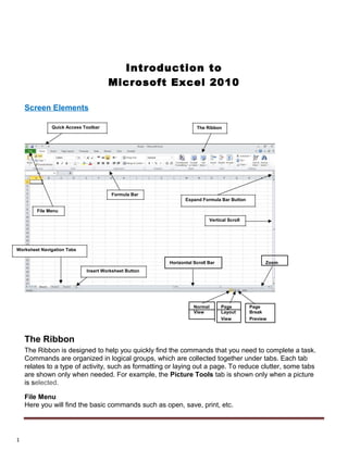
1. Introduction to
Microsoft Excel 2010
Screen Elements
Quick Access Toolbar
Formula Bar
File Menu
Worksheet Navigation Tabs
Insert Worksheet Button
The Ribbon
Expand Formula Bar Button
Vertical Scroll
ZoomHorizontal Scroll Bar
Normal Page Page
View Layout Break
View Preview
The Ribbon
The Ribbon is designed to help you quickly find the commands that you need to complete a task.
Commands are organized in logical groups, which are collected together under tabs. Each tab
relates to a type of activity, such as formatting or laying out a page. To reduce clutter, some tabs
are shown only when needed. For example, the Picture Tools tab is shown only when a picture
is selected.
File Menu
Here you will find the basic commands such as open, save, print, etc.
1

2. Quick Access Toolbar
The place to keep the items that you not only need to access quickly, but want to be immediately
available regardless of which of the Ribbon's tabs you're working on. If you put so many items on
the Quick Access Toolbar that it becomes too big to fit on the title bar, you can move it onto its
own line.
Formula Bar
A place where you can enter or view formulas or text.
Expand Formula Bar Button
This button allows you to expand the formula bar. This is helpful when you have either a long
formula or large piece of text in a cell.
Worksheet Navigation Tabs
By default, every workbook has 3 sheets. You are able to navigate the sheets by clicking on the
sheet tab.
Insert Worksheet Button
Click the Insert New Worksheet button to insert a new worksheet in your workbook.
Normal View
This is the “normal view” for working on a spreadsheet in Excel.
Page Layout View
View the document as it will appear on the printed page.
Page Break Preview
View a preview of where pages will break when the document is printed.
Zoom Level
Allows you to quickly zoom in or zoom out of the worksheet.
Horizontal/Vertical Scroll
Allows you to scroll vertically/horizontally in the worksheet.

3. Highlighting/Selecting Areas Using the Mouse
Select Cells:
Moves a cell’s contents:
Activate the Auto fill feature:
.
To Select a Column: Click on the column letter
To Select a Row: Click on the row number
To Select the Entire Worksheet: Click above row 1 and to the left of column A or hit CTRL A on
the keyboard

4. Creating Formulas
Formulas perform calculations or other actions on the data in your worksheet. A formula starts with
an equal sign (=). It is possible to create formulas in Excel using the actual values, such as
“4000*.4” but it is more beneficial to refer to the cell address in the formula, for example “D1*.4”.
One of the benefits of using a spreadsheet program is the ability to create a formula in one cell and
copy it to other cells. Most spreadsheet formulas use a concept called relative referencing.
This is the explanation of relative referencing from Excel’s help file:
“A relative cell reference in a formula, such as A1, is based on the relative position of the cell that
contains the formula and the cell the reference refers to. If the position of the cell that contains the
formula changes, the reference is changed. If you copy the formula across rows or down columns,
the reference automatically adjusts. By default, new formulas use relative references. For
example, if you copy a relative reference in cell B2 to cell B3, it automatically adjusts.”
It is also important to know the operators Excel uses for formulas:
Operator (Key) Function
= Begins all Excel functions and formulas
+ Addition
- Subtraction
* Multiplication
/ Division
To Create a Formula:
1) Click in a cell
2) Press the = key
3) Type the formula
4) Press Enter
Copying Formulas
Like many things in Excel, there is more than one way to copy formulas. Feel free to choose what
works best for you.
To Copy Formulas Using Autofill:
1) Click in the cell that contains the formula
2) Position the mouse on the Autofill handle (a thin black cross will appear)
3) Click and drag to copy the formula

5. To Copy Formulas Using Copy and Paste:
1) Click in the cell that contains a formula
2) Select Copy on the Home Ribbon in the Editing group
3) Highlight the cell where you would like to paste the formula
4) Select Paste on the Home Ribbon in the Editing group
ALTERNATE METHODS
Keyboard: Ribbon: Mouse:
Press CTRL + C Right-click and choose
Copy
Auto sum Function
To Create the Total Column’s Values Using Autosum:
1) Click in the cell where you would like the Total to be located
2) Press the Autosum button on the Home Ribbon
The Autosum function automatically looks for cells that have values in them. It will read values
until it finds the first blank cell. Autosum will always look for values in the cells above it first, then to
the left. This means that you need to be aware of what cells will be in the formula. Autosum will
select the range of cells to use in the formula by highlighting the range.
3) Press Enter
Saving a Worksheet
When working in Excel it is necessary to save your files. It is also very important that while
working, your file is saved frequently. When naming a file, you are restricted to 255 characters.
Avoid most punctuation; spaces are acceptable.

6. To Save the File:
1) Click on the File tab
2) Click Save
3) Type a file name
4) Click Save
Clearing Cells
As we begin to look at formatting, it is important to understand what makes up the contents of
a cell. There are three distinct items that can be in a cell:
• Contents
• Formats
• Comments
To Clear a Cell Format:
1) Click in the cell that contains formatting
2) Click the drop-down arrow next to the Clear button on the Home tab in the Editing group
3) Click Clear Formats
Formatting Values
Applying formats to any cell(s) can be done either using the Font, Alignment and Number
groups or using the dialog box which will include all the formatting options.
To Apply the Currency Format:
1) Highlight the cells
2) Click on the Currency Style button on the Home tab in the Number group
3) If necessary, click on the Increase or Decrease Decimal button on the Number group

7. To Apply the Comma Format:
1) Highlight cells
2) Click on the Comma Style button on the Number group
3) If necessary, click on the Increase or Decrease Decimal button on the Number group
Formatting Labels
A Label, or text formatting is applied virtually the same way it is done in word processing
programs.
To Format the Title Labels:
1) Highlight the cell(s)
2) Select a font from the Font group
3) Select a point size from the Font group
Using the Dialog Box:
1) Highlight the cells
2) Click on the arrow in the corner of one of the formatting groups (Font, Alignment, Number)
to open the Format Cells dialog box and click on one of the tabs

8. Format Painter
Frequently, you will need to take a format that is applied to one cell and apply it to other cells. A
quick way to do this is by using the Format Painter .
To Apply a Format to Cells:
1) Highlight cell(s)
2) Format the cell(s) to the desired format
3) Select the formatted cell(s)
4) Click the Format Painter from the Clipboard group of the Home tab
5) Highlight the cells you wish to format
Tips and Tricks: If you would like the Format Painter to remain active, double-click the Format
Painter. It will remain active until you press the Esc key.
To Change a Cell’s Alignment:
1) Highlight the cell(s)
2) Click the orientation button on the Alignment group
3) Select an alignment
Centering Text Across Columns
When it comes to titles, it may be preferable to have the information centered across the
document, rather than in only one cell. Excel uses the feature Merge Cells to accomplish this.
To Center the Title Across Columns:
1) Highlight cell(s)
2) Click the Merge and Center button on the Alignment group
NOTE: Each cell must be done individually. Excel will delete the contents of all but the top
most cell if multiple cells are selected.
This option basically takes all the cells in the highlighted range and merges them into one large
cell. For example, the range A1:F1 became cell A1 after the Merge Cells button was selected.
There is no cell B1, C1, etc. any longer.

9. Creating a Basic Chart
1) Highlight the data to be charted
2) Click on the Insert tab
3) Click on a Chart Type in the Charts group
4) Click on a Chart Style
To Move your Chart:
Click and drag the chart to a new location on the worksheet.
When the chart is selected you will notice a new tab “Chart Tools” on the Ribbon. If you do not
see the Chart Tools, click on the chart to select it. Under Chart Tools you will find 3 tabs:
• Design
• Layout
• Format

10. Excel Functions
As we have previously seen, the power of Excel lies in its ability to perform calculations. The real
strength of this is shown in Functions. Functions are more complex formulas that are executed by
using the name of a function and stating whatever parameters the function requires.
Function Defined
=SUM(range of cells) returns the sum of the selected cells
=AVERAGE (range of cells) returns the average of the selected cells
=MAX(range of cells) returns the highest value of the selected cells
=MIN(range of cells) returns the lowest value of the selected cells
=COUNT(range of cells) returns the number of values of the selected cells
To Enter the SUM Function:
1) Click in a cell
2) Click on the AutoSum button in the Editing group
3) Highlight the range of cells that are to be added (The colon means “through”)
4) Press ENTER
1) Click in a cell
2) Click on the drop-down arrow next to the AutoSum button
3) Click on Average
4) Highlight the range of cells be calculated
5) Press ENTER

11. To Insert the MAX Function into the Worksheet:
1) Click in a cell
2) Click on the drop-down arrow next to the AutoSum button
3) Click on Max
4) Highlight the range of cells be calculated
5) Press ENTER
1) Click in a cell
2) Click on the drop-down arrow next to the AutoSum button
3) Click on Min
4) Highlight the range of cells be calculated
5) Press ENTER
1) Click in a cell
2) Click on the drop-down arrow next to the AutoSum button
3) Click on Count Numbers
4) Highlight the range of cells be calculated
5) Press ENTER
Printing a Worksheet
To Print, Preview and Modify Page Setup
1) Click on the File tab
2) Click on Print
The spreadsheet shows as it will be printed. You can proceed to print the document from here, or
you can change things to make the printed output look different.
14

12. Page Setup
You can change options under Settings or you can click on Page Setup.
Clicking on Page Setup will open a dialog box with four tabs:
• Page
• Margins
• Header/Footer
• Sheet
Page Options:
1) Change the Orientation
2) Adjust the Scaling
3) Change the Paper Size
Margins:
1) Change the margins
2) Center on the page either horizontally, vertically or select both
Header/Footer:
1) To select from one of the already created headers/footers, click on the drop-down arrow for
Header and also for Footer and choose from the list
2) To create a custom header and/or footer, click on Custom Header and Custom Footer