In this project, we used the Capital Assets Pricing Model (CAPM) to test for the ‘January effect’ - a calendar‐related market anomaly in the financial market where financial security prices increase in the month of January. Please refer to "Chapter 2 – The Capital Asset Pricing Model: An Application of Bivariate Regression Analysis" of the book "The Practice of Econometrics" by Ernst R. Bernd for the test data, background and problem statement.

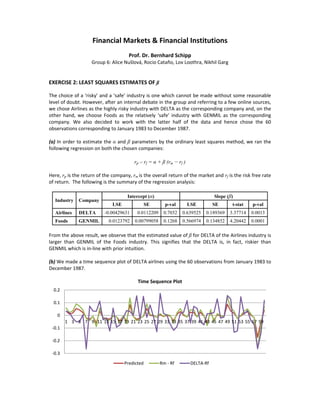
1. Financial Markets & Financial Institutions
Prof. Dr. Bernhard Schipp
Group 6: Alice Nušlová, Rocio Cataño, Lov Loothra, Nikhil Garg
EXERCISE 2: LEAST SQUARES ESTIMATES OF ß
The choice of a ‘risky’ and a ‘safe’ industry is one which cannot be made without some reasonable
level of doubt. However, after an internal debate in the group and referring to a few online sources,
we chose Airlines as the highly risky industry with DELTA as the corresponding company and, on the
other hand, we choose Foods as the relatively ‘safe’ industry with GENMIL as the corresponding
company. We also decided to work with the latter half of the data and hence chose the 60
observations corresponding to January 1983 to December 1987.
(a) In order to estimate the α and ß parameters by the ordinary least squares method, we ran the
following regression on both the chosen companies:
rp – rf = α + ß (rm − rf )
Here, rp is the return of the company, rm is the overall return of the market and rf is the risk free rate
of return. The following is the summary of the regression analysis:
Industry Company
Intercept (α) Slope (ß)
LSE SE p-val LSE SE t-stat p-val
Airlines DELTA -0.00429631 0.0112209 0.7032 0.639525 0.189369 3.37714 0.0013
Foods GENMIL 0.0123792 0.00799058 0.1268 0.566974 0.134852 4.20442 0.0001
From the above result, we observe that the estimated value of ß for DELTA of the Airlines industry is
larger than GENMIL of the Foods industry. This signifies that the DELTA is, in fact, riskier than
GENMIL which is in‐line with prior intuition.
(b) We made a time sequence plot of DELTA airlines using the 60 observations from January 1983 to
December 1987.
Time Sequence Plot
‐0.3
‐0.2
‐0.1
0
0.1
0.2
1 3 5 7 9 11 13 15 17 19 21 23 25 27 29 31 33 35 37 39 41 43 45 47 49 51 53 55 57 59
Predicted Rm ‐ Rf DELTA‐Rf

2. From the unusual residual data, the value corresponding to observation 7 (July 1983) had a
studentized residual value of ‐3.07, a residual of ‐0.246406 and a corresponding value of ‐0.26614
(the least value). Upon inspecting the historical data, the value can be accounted for by the July 17,
1983 hijacking of Delta 722 Miami‐Tampa 727.
Furthermore, if we observe the value corresponding to observation 58, it is nearly as low as
observation 7. However, it is not an outlier! This is because that value corresponds to the Black
Monday Crash of October 19, 1987 which is accounted for in the market variable as well.
(c) We now test for the following hypothesis:
H0: α = 0
Ha: α ≠ 0
From the regression analysis summary in part (a), we can observe that the p‐values for all
observations are greater than 0.05. Hence, at the 95% confidence level, we cannot reject the null
hypothesis that H0: α = 0. α does not play a significant role in CAPM and is only used to fit the
regression.
(d) We now prepare the 95% confidence intervals for DELTA and GENMIL. From the statistics we
obtained in part (a), we have the following:
DELTA: 0.639525 ± 0.378738 => 0.260787 to 1.018263
GENMIL: 0.566974 ± 0.269704 => 0.29727 to 0.836678
We now test for the following hypothesis:
H0: ß = 1
Ha: ß ≠ 1
Now, in this case, the t‐value is given by: t-stat = (ß – 1) / SE (ß); where SE is the Standard Error.
Hence, the t‐test value for DELTA is –1.903558 and for GENMIL it is –3.211120. The corresponding p‐
values for two‐tailed and one‐tailed tests are given below:
p-value (two-tailed t-test) p-value (one-tailed t-test)
DELTA 0.0618 0.0309
GENMIL 0.0021 0.00105
For GENMIL we can reject H0 but the same is not possible for DELTA. This is because the p‐value for
the two‐tailed t‐test is greater than 0.05. There are no surprises here.
(e) The proportion of stock that is non‐diversifiable is given by the R2
statistic from the regression
analysis we did in part (a). For DELTA, the R2
statistic is 16.4326%. Hence the proportion of stock that
is non‐diversifiable for DELTA is 16.4326% and the proportion that is diversifiable is 83.5674%.
Similarly, for GENMIL, the R2
statistic is 23.3586% which determines the proportion of stock that is
non‐diversifiable. Thus the proportion that is diversifiable is 76.6414%. In both the cases, the
proportion which is non‐diversifiable is less than a typical stock.
The results are not surprising. GENMIL and DELTA are both less diversified in the market, so even
though these stocks do move with the market, they have a large proportion of “company‐specific”
risk.

3. (f) From our sample data, we have the following observations:
DELTA: ß = 0.639525 & R2
= 16.4326%
GENMIL: ß = 0.566974 & R2
= 23.3586%
Hence in our sample data, a large value of ß does not necessarily correspond with a higher R2
value.
Given that R2 is defined as R2
= ß2
σm
2
/(ß2
σm
2
+ σε
2
), the relationship would be exact if firms have
roughly similar firm‐specific risk. However, as observed above, this is not the case for our sample.
EXERCISE 8: IS JANUARY DIFFERENT?
There is some tentative evidence which supports the notion that stock returns in the month of
January are relatively higher. This is referred to as the “January Effect”, a calendar‐related market
anomaly in the financial market where financial security prices increase in the month of January. This
effect was first observed by investment banker Sidney B. Wachtel.
This creates an opportunity for investors to buy stock for lower prices before January and sell them
after their value increases. This effect is curious because even if we consider investors selling losing
stocks in December, the expectation of higher January returns should shift supply‐demand curves
and equilibrate returns.
We will try to empirically and statistically test this hypothesis in our report.
(a) If the “January premium” affected the overall market return rm and the risk‐free return rf by the
same amount jm, the market risk premium, MRP, would be:
MRP = r'm – r'f = (rm + jm) – (rf + jm)
= rm – rf + jm – jm
= rm – rf
Therefore, the market risk premium would not be affected by the January premium.
We will now try and ascertain whether the “January is different” hypothesis be tested within the
CAPM framework of Eq. (2.17). The estimable equation relating the total risk premium of security, j,
to the market risk premium and to the stochastic disturbance term is:
rj – rf = αj + ßj (rm – rf) + εj
We conclude, therefore, that the hypothesis cannot be tested within the CAPM framework, because
the independent variable of the regression, that is, the market risk premium, would be unchanged.
Furthermore, we believe that it would not be more reasonable to assume that the “January is
different” hypothesis referred only to risky assets because if January is actually different, the returns
of all stocks (including the risk‐free returns) should differ and not just risky assets.
(b) If r'm = rm + jm and the risk‐free assets return is unaffected, then the market risk premium, MRP,
would be:
MRP = r'm – rf = rm + jm – rf
Therefore, the market risk premium would be affected.

4. Furthermore, if the CAPM model were true and the α and ß parameters were constant, then the
expected portfolio return would be:
r'p = rf + α + ß (r'm – rf)
=> r'p = rf + α + ß (rm + jm – rf)
=> r'p = rf + α + ß (rm – rf) + ß jm
Now since, rf + α + ß (rm – rf) = rp, our equation becomes:
r'p ≡ rp + ß jm
Now, re‐writing the CAPM regression equation using the right‐hand sides of the above expressions,
we get:
r'p – rf = α + ß (r'm – rf ) + ε
=> rp + ß jm – rf = α + ß (rm + jm – rf) + ε
= α + ß (rm – rf ) +ß jm + ε
Now, considering the term ß jm to be unobservable, we subtract it from both the sides to get:
rp – rf = α + ß (rm – rf) + ε
Comparing the above equation with Eq. 2.17, we observe that the equation has reduced to the
original CAPM equation sans the January premium. With this we therefore conclude that we cannot
estimate the “January premium” within the CAPM framework under these assumptions as well.
(c) From the conclusions drawn from parts (a) and (b), we now abandon the CAPM model and
examine an alternative method of testing the “January is different” hypothesis. We decided to
choose the following industries and their corresponding companies: Computers (IBM and DATGEN),
Foods (GERBER and GENMIL) and Banks (CONTIL and CITCRP).
For each of these companies we ran the following regression:
rp = α + ß (DUMJ)
Here, rp is the return of the company, and DUMJ is a dummy variable, which takes the value of unity
if the month is January and zero for all other months. The following is the summary of the regression
analysis:
Industry Company
Intercept Slope (DUMJ)
LSE SE p-val LSE SE t-stat p-val
Computers
IBM 0.00817273 0.005633 0.1495 0.017327 0.019512 0.888016 0.3763
DATGEN 0.00405455 0.012163 0.7395 0.041146 0.042133 0.976555 0.3308
Foods
GERBER 0.0157636 0.008398 0.063 0.007636 0.029093 0.262482 0.7934
GENMIL 0.0170909 0.006225 0.007 -0.00609 0.021566 -0.28244 0.7781
Banks
CONTIL -0.0064818 0.014327 0.6518 0.064582 0.04963 1.30127 0.1957
CITCRP 0.0118455 0.007753 0.1292 0.000155 0.026857 0.005754 0.9954

5. The above table gives the values of the estimated regression parameters (LSE = Least Squares
Estimate, which is the coefficient), the standard error (SE) of the estimate, the corresponding p‐
values for the slope and the intercept and the t‐statistic for the slope.
Now we test the null hypothesis that the coefficient on the DUMJ variable is zero against the
alternative hypothesis that it is not zero. We therefore have:
H0: ß = 0
Ha: ß ≠ 0
If we use a 5% significance level or a 95% confidence interval, we cannot reject H0 that the
coefficient on the DUMJ variable is zero for any of the chosen companies. For each of the chosen
companies, the p‐value is larger than 0.05. Furthermore, the critical value of the t‐distribution for a
two‐sided test with 95% confidence interval is 1.98 for 120 observations (since we’re working on 120
months in total). Therefore, we can make an equivalent observation that the t‐statistic for the
DUMJ variable is less than 1.98 for all companies.
Based on these results and the reasonable 5% significance level, we conclude that January is not
different.
(e) We now move on to yet another way of examining the “January is different hypothesis”. In this
part of the exercise, we use the risk premiums of the various companies we chose in part (c) (rp – rf),
the market premium (rm – rf) and the DUMJ variable which is unity whenever the observation
corresponds to the month of January and zero otherwise. We then ran the following regression for
every company:
rp – rf = α + ß1(DUMJ) + ß2(rm – rf) + ε
By doing this, we have restricted the slope coefficients to be the same for all months but have
allowed the intercept term for January to be different from the common intercept for the other
months. The following is the summary of the regression analysis:
Industry Company
Intercept DUMJ Marker Risk Premium
LSE p-val LSE t-stat p-val LSE p-val
Computers
IBM -0.001173 0.8093 0.008424 0.501443 0.617 0.454218 0.0000
DATGEN -0.0084713 0.4102 0.02148 0.605076 0.5463 1.02418 0.0000
Foods
GERBER 0.00545394 0.462 -0.00453 -0.17696 0.8598 0.626992 0.0000
GENMIL 0.00875192 0.148 -0.01159 -0.5566 0.5789 0.273791 0.0015
Banks
CONTIL -0.0172848 0.207 0.050747 1.07557 0.2843 0.715408 0.0003
CITCRP 0.00129034 0.8415 -0.01284 -0.57597 0.5657 0.670978 0.0000
Now, we will use the above results to test for the null hypothesis that “January is different”. Now, in
this case, the said hypothesis can be considered to be equivalent to rejecting the null hypothesis that
ß1 is zero. Therefore, we have:
H0: ß1 = 0
Ha: ß1 ≠ 0
If we use a 5% significance level and check the p‐values of the DUMJ variable, we observe that we
cannot reject the null hypothesis that ß1 is zero for all the chosen companies. This is because for

6. each of the observations, the p‐value is larger than 0.05 and, equivalently, the t‐statistic is smaller
than 1.98 (which, as discussed in part (c) above, is the critical value of the t‐distribution for 120
observations at 95% confidence level). We therefore conclude that the intercept in the CAPM
regression is the same for January and the remaining 11 months of the year. As can be observed, the
common intercept for the remaining months of the year is not significantly different from zero in
every regression.
We now use the above results to test the null hypothesis that “January is better”. In this situation,
the said hypothesis corresponds to a one‐sided test for the DUMJ variable. Therefore, we have:
H0: ß1 = 0
Ha: ß1 > 0
In this test, we use the t‐statistic of the ß1 parameter and compare each of the observations with
1.658, which is the critical value for 120 observations from the t‐distribution at the 95% confidence
level for a one‐sided test. We can observe from our table of results that the t‐statistic is less than
1.658 in all the cases.
We therefore conclude that the “January is better” hypothesis is false for all our chosen companies.
(f) From the above analysis, we can conclude that January is not different.
We assumed in part (a) that the “January premium” affected the returns of both the risk‐free and
the risky assets. In part (b), we assumed that the premium affected only the risky assets returns.
However, as observed in both parts (a) and (b), if a “January premium” does exist, it cannot be
tested for within the CAPM framework.
We investigated an alternative methodology of testing the “January is different” hypothesis in part
(c) by using 6 companies from 3 different industries (viz. Computers, Foods and Banks). By
introducing a dummy variable for January (DUMJ) and running the regression: rp = α + ß (DUMJ),
we rejected the hypothesis that “January is different” at 5% significance level for every company.
In part (e) we investigated yet another way of analyzing the given hypothesis by allowing for a
difference only in the intercept term within the CAPM framework. By running the regression: rp – rf
= α + ß1(DUMJ) + ß2(rm – rf) + ε and analyzing the subsequent results, we concluded that at a 95%
confidence interval, the intercept does not change significantly in January for all the chosen
companies.
Hence, based on the results in each part of the given exercise we are in a position to conclude that
the returns and the risk‐premiums are not significantly different in January as compared to the other
months of the year, i.e., January is not different.

7. APPENDIX
Programming Package used: STATGRAPHICS Centurion XVI, Microsoft Excel 2010
Sample regression analysis summary for Exercise 2, Part (a):
Regression: rp – rf = α + ß (rm − rf ) for Delta:
Simple Regression - delta_last_60-Rf vs. Rm-Rf
Dependent variable: delta_last_60-Rf
Independent variable: Rm-Rf
Linear model: Y = a + b*X
Coefficients
Least Squares Standard T
Parameter Estimate Error Statistic P-Value
Intercept -0.00429631 0.0112209 -0.382883 0.7032
Slope 0.639525 0.189369 3.37714 0.0013
Analysis of Variance
Source Sum of Squares Df Mean Square F-Ratio P-Value
Model 0.0859235 1 0.0859235 11.41 0.0013
Residual 0.43696 58 0.00753379
Total (Corr.) 0.522883 59
Correlation Coefficient = 0.405372
R-squared = 16.4326 percent
R-squared (adjusted for d.f.) = 14.9918 percent
Standard Error of Est. = 0.0867974
Mean absolute error = 0.0681243
Durbin-Watson statistic = 2.16048 (P=0.7273)
Lag 1 residual autocorrelation = -0.0871333
The StatAdvisor
The output shows the results of fitting a linear model to describe the relationship between
delta_last_60-Rf and Rm-Rf. The equation of the fitted model is
delta_last_60-Rf = -0.00429631 + 0.639525*Rm-Rf
Since the P-value in the ANOVA table is less than 0.05, there is a statistically significant relationship
between delta_last_60-Rf and Rm-Rf at the 95.0% confidence level.
The R-Squared statistic indicates that the model as fitted explains 16.4326% of the variability in
delta_last_60-Rf. The correlation coefficient equals 0.405372, indicating a relatively weak
relationship between the variables. The standard error of the estimate shows the standard deviation of
the residuals to be 0.0867974. This value can be used to construct prediction limits for new
observations by selecting the Forecasts option from the text menu.
The mean absolute error (MAE) of 0.0681243 is the average value of the residuals. The Durbin-
Watson (DW) statistic tests the residuals to determine if there is any significant correlation based on
the order in which they occur in your data file. Since the P-value is greater than 0.05, there is no
indication of serial autocorrelation in the residuals at the 95.0% confidence level.

8. Sample regression analysis summary for Exercise 8, Part (c):
Regression: rp = α + ß (DUMJ) for Continental Illinois:
Simple Regression - contil vs. DUMJ
Dependent variable: contil
Independent variable: DUMJ
Linear model: Y = a + b*X
Coefficients
Least Squares Standard T
Parameter Estimate Error Statistic P-Value
Intercept -0.00648182 0.0143269 -0.452422 0.6518
Slope 0.0645818 0.04963 1.30127 0.1957
Analysis of Variance
Source Sum of Squares Df Mean Square F-Ratio P-Value
Model 0.0382324 1 0.0382324 1.69 0.1957
Residual 2.66429 118 0.0225787
Total (Corr.) 2.70252 119
Correlation Coefficient = 0.118941
R-squared = 1.4147 percent
R-squared (adjusted for d.f.) = 0.579227 percent
Standard Error of Est. = 0.150262
Mean absolute error = 0.0875947
Durbin-Watson statistic = 1.93443 (P=0.3605)
Lag 1 residual autocorrelation = 0.0256169
The StatAdvisor
The output shows the results of fitting a linear model to describe the relationship between contil and
DUMJ. The equation of the fitted model is
contil = -0.00648182 + 0.0645818*DUMJ
Since the P-value in the ANOVA table is greater or equal to 0.05, there is not a statistically significant
relationship between contil and DUMJ at the 95.0% or higher confidence level.
The R-Squared statistic indicates that the model as fitted explains 1.4147% of the variability in contil.
The correlation coefficient equals 0.118941, indicating a relatively weak relationship between the
Plot of Fitted Model
delta_last_60-Rf = -0.00429631 + 0.639525*Rm-Rf
-0.27 -0.17 -0.07 0.03 0.13 0.23
Rm-Rf
-0.27
-0.17
-0.07
0.03
0.13
0.23
delta_last_60-Rf

9. variables. The standard error of the estimate shows the standard deviation of the residuals to be
0.150262. This value can be used to construct prediction limits for new observations by selecting the
Forecasts option from the text menu.
The mean absolute error (MAE) of 0.0875947 is the average value of the residuals. The Durbin-
Watson (DW) statistic tests the residuals to determine if there is any significant correlation based on
the order in which they occur in your data file. Since the P-value is greater than 0.05, there is no
indication of serial autocorrelation in the residuals at the 95.0% confidence level.
Sample regression analysis summary for Exercise 8, Part (e):
Regression: rp – rf = α + ß1(DUMJ) + ß2(rm – rf) + ε for Citicorp
Multiple Regression - citicrp-rkfree
Dependent variable: citicrp-rkfree
Independent variables:
DUMJ
market-rkfree
Standard T
Parameter Estimate Error Statistic P-Value
CONSTANT 0.00129034 0.00643722 0.20045 0.8415
DUMJ -0.0128418 0.0222961 -0.575967 0.5657
market-rkfree 0.670978 0.0901989 7.43887 0.0000
Analysis of Variance
Source Sum of Squares Df Mean Square F-Ratio P-Value
Model 0.250693 2 0.125346 27.67 0.0000
Residual 0.530045 117 0.0045303
Total (Corr.) 0.780738 119
R-squared = 32.1097 percent
R-squared (adjusted for d.f.) = 30.9492 percent
Standard Error of Est. = 0.0673075
Mean absolute error = 0.0518742
Durbin-Watson statistic = 1.84745 (P=0.2028)
Lag 1 residual autocorrelation = 0.0708349
Plot of Fitted Model
contil = -0.00648182 + 0.0645818*DUMJ
0 0.2 0.4 0.6 0.8 1
DUMJ
-0.6
-0.2
0.2
0.6
1
contil

10. The StatAdvisor
The output shows the results of fitting a multiple linear regression model to describe the relationship
between citicrp-rkfree and 2 independent variables. The equation of the fitted model is
citicrp-rkfree = 0.00129034 - 0.0128418*DUMJ + 0.670978*market-rkfree
Since the P-value in the ANOVA table is less than 0.05, there is a statistically significant relationship
between the variables at the 95.0% confidence level.
The R-Squared statistic indicates that the model as fitted explains 32.1097% of the variability in
citicrp-rkfree. The adjusted R-squared statistic, which is more suitable for comparing models with
different numbers of independent variables, is 30.9492%. The standard error of the estimate shows
the standard deviation of the residuals to be 0.0673075. This value can be used to construct prediction
limits for new observations by selecting the Reports option from the text menu. The mean absolute
error (MAE) of 0.0518742 is the average value of the residuals. The Durbin-Watson (DW) statistic
tests the residuals to determine if there is any significant correlation based on the order in which they
occur in your data file. Since the P-value is greater than 0.05, there is no indication of serial
autocorrelation in the residuals at the 95.0% confidence level.
In determining whether the model can be simplified, notice that the highest P-value on the
independent variables is 0.5657, belonging to DUMJ. Since the P-value is greater or equal to 0.05,
that term is not statistically significant at the 95.0% or higher confidence level. Consequently, you
should consider removing DUMJ from the model.
REFERENCES
[1] Berndt, "The Practice of Econometrics; Chapter 2 – The Capital Asset Pricing Model: An
Application of Bivariate Regression Analysis”
[2] Prof. Dr. Bernhard Schipp, Course Script: “Financial Markets and Financial Institutions
(Essentials of Quantitative Finance)”
Plot of citicrp-rkfree
-0.29 -0.09 0.11 0.31 0.51
predicted
-0.29
-0.09
0.11
0.31
0.51
observed