Regression analysis measures the average relationship between two or more variables using their original data units. There are two main types: simple regression involving two variables, and multiple regression involving more than two variables. Regression can be linear, following a straight line, or non-linear/curvilinear. A simple linear regression model relates a dependent variable Y to an independent variable X plus an error term. Estimating the model involves calculating the slope/regression coefficient and intercept. Multiple regression relates a dependent variable to two or more independent variables using a multiple correlation coefficient.

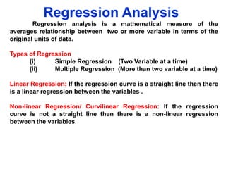
1. Regression Analysis
Regression analysis is a mathematical measure of the
averages relationship between two or more variable in terms of the
original units of data.
Types of Regression
(i)
Simple Regression (Two Variable at a time)
(ii)
Multiple Regression (More than two variable at a time)
Linear Regression: If the regression curve is a straight line then there
is a linear regression between the variables .
Non-linear Regression/ Curvilinear Regression: If the regression
curve is not a straight line then there is a non-linear regression
between the variables.

2. Simple Linear Regression Model & its Estimation
A simple linear regression model is based on a single independent
variable and its general form is:
Yt     X t   t
Here
Intercepts
Yt
Xt
t
= dependent variable or regressands
= independent variable or regressor
= random error or disturbance term
Importance of error
(i)
Slope/ Regression Coefficients
 t term:
It captures the effect of on the dependent variable of all
variable not included in the model.
(ii) It captures any specification error related to assumed linear
functional form.
(iii) It captures the effects of unpredictable random componenets
present in the dependent variable.

3. Estimation of the Model
Yt
Xt
Sales
Adver Exp
(thousands (million of
of Unit)
Rs.)
ˆ
Yt
ˆ
X
=309/
7
36/7
t
xt2
y t  Y t  Yˆt
ˆ
xt  X t  X t
xtyt
-7.14286
-0.64286
4.591837
0.413265
37
4.5
48
6.5
3.857143
1.357143
5.234694
1.841837
45
3.5
0.857143
-1.64286
-1.40816
2.69898
36
3
-8.14286
-2.14286
17.44898
4.591837
25
2.5
-19.1429
-2.64286
50.59184
6.984694
55
8.5
10.85714
3.357143
36.44898
11.27041
63
7.5
18.85714
2.357143
44.44898
5.556122
44.1428
∑Yt =309
∑Xt = 36
5.1428
∑xt yt
=157.37
∑xt 2 =
33.354

4. Estimation of the Model
ˆ
 
xy
x
t
2
t
t

157 . 357
 4 . 717
33 . 354
ˆˆ
ˆ
  Y   X  44 . 143  ( 4 . 717 )( 5 . 143 )  19 . 882
ˆ
Then the estimated simple linear regression model is
Y t  19 . 882  4 . 717 X t

11. ˆ
2 
x y
x
2
2
t
t

157 . 357
 4 . 717
33 . 354
ˆˆ
ˆ
  Y   X  44 . 143  ( 4 . 717 )( 5 . 143 )  19 . 882
ˆ
Y t  19 . 882  4 . 717 X t

16. General Formula for First Order Coefficients
rYX .W 
rXY  rXW rYW
(1  rXW )(1  rYW )
2
2
General Formula for Second Order Coefficients
rYX .WO 
rXY .O  rXW .O rYW .O
(1  r
2
XW . O
)(1  r
2
YW . O
)

17. Partial Correlation
Remarks:
1. Partial correlation coefficients lies between -1 & 1
2. Correlation coefficients are calculated on the bases of zero
order coefficients or simple correlation where no variable is
kept constant.
Limitation:
1. In the calculation of partial correlation coefficients, it is
presumed that there exists a linear relation between variables.
In real situation, this condition lacks in some cases.
2. The reliability of the partial correlation coefficient decreases as
their order goes up. This means that the second order partial
coefficients are not as dependable as the first order ones are.
Therefore, it is necessary that the size of the items in the gross
correlation should be large.
3. It involves a lot of calculation work and its analysis is not easy.

18. Partial Correlation
Example: From the following data calculate 12.3
x1 : 4
0
1
1
1
3
x2 : 2
0
2
4
2
3
x3 : 1
4
2
2
3
0
Solution:
X
1

16
2
 2,
X
2

16
2
 2
and
X
3

16
2
 2
4
1
3
0
4
0

19. Partial Correlation

20. Multiple Correlation
The fluctuation in given series are not usually dependent upon a
single factor or cause. For example wheat yields is not only
dependent upon rain but also on the fertilizer used, sunshine etc.
The association between such series and several variable causing
these fluctuation is known as multiple correlation.
It is also defined as “ the correlation between several variable.”
Co-efficient of Multiple Correlation:
Let there be three variable X1, X2 and X3.
Let X1 be dependent variable, depending upon independent
variable , X2 and X3. The multiple correlation coefficient are defined
as follows:
R1.23 = Multiple correlation with X1 as dependent variable and X2. and X3. , as
independent variable
R2.13 = Multiple correlation with X2 as dependent variable and X1. and X3. , as
independent variable
R3.12 = Multiple correlation with X3 as dependent variable and X1. and X2 , as
independent variable

21. Calculation of Multiple Correlation Coefficient
General Formula
For example

22. Remarks
•
•
•
•
•
•
•
Multiple correlation coefficient is a non-negative coefficient.
It is value ranges between 0 and 1. It cannot assume a minus
value.
If R1.23 = 0, then r12 = 0 and r13=0
R1.23 r12 and R1.23 r13
R1.23 is the same as R1.32
(R1.23 )2 = Coefficient of multiple determination.
If there are 3 independent variable and one dependent variable the
formula for finding out the multiple correlation is
R1 .234 
1  (1  r
2
14 )(1  r
2
12 . 3 )(1  r
2
12 . 34
)

23. Limitation

24. Advantages of Multiple Correlation

25. Example
Given the following data
X1:
3
5
X2:
16
10
X3:
90
72
6
7
54
8
4
42
12
3
30
Compute coefficients of correlation of X3 on X1 and X2
14
2
12

26. Example

27. Example

28. Types of Correlation
r12.3 is the correlation between variables 1 and 2 with variable 3
removed from both variables. To illustrate this, run separate
regressions using X3 as the independent variable and X1 and X2 as
dependent variables. Next, compute residuals for regression...
X