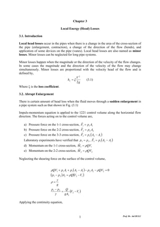
1. Chapter 3
Local Energy (Head) Losses
3.1. Introduction
Local head losses occur in the pipes when there is a change in the area of the cross-section of
the pipe (enlargement, contraction), a change of the direction of the flow (bends), and
application of some devices on the pipe (vanes). Local head losses are also named as minor
losses. Minor losses can be neglected for long pipe systems.
Minor losses happen when the magnitude or the direction of the velocity of the flow changes.
In some cases the magnitude and the direction of the velocity of the flow may change
simultaneously. Minor losses are proportional with the velocity head of the flow and is
defined by,
V2
hL = ξ (3.1)
2g
Where ξ is the loss coefficient.
3.2. Abrupt Enlargement
There is certain amount of head loss when the fluid moves through a sudden enlargement in
a pipe system such as that shown in Fig. (3.1)
Impuls-momentum equation is applied to the 1221 control volume along the horizontal flow
direction. The forces acting on to the control volume are,
r
a) Pressure force on the 1-1 cross-section, F1 = p1 A1
s
b) Pressure force on the 2-2 cross-section, F2 = p2 A2
r
c) Pressure force on the 3-3 cross-section, F3 = p3 ( A2 − A1 )
r
Laboratory experiments have verified that p3 = p1 , F3 = p1 ( A2 − A1 )
r
d) Momentum on the 1-1 cross-section, M 1 = ρQV1
r
e) Momentum on the 2-2 cross-section, M 2 = ρQV2
Neglecting the shearing force on the surface of the control volume,
ρQV1 + p1 A1 + p1 ( A2 − A1 ) − p 2 A2 − ρQV2 = 0
( p1 − p2 )A2 = ρQ(V2 − V1 )
γ
ρ=
g
p1 − p 2
=
Q
(V2 − V1 )
γ gA2
Applying the continuity equation,
1 Prof. Dr. Atıl BULU

2. Energy Line (V1 − V2 )2
hL =
2g
V 22
V12
2g
2g
H.G.L
p2
p1
γ
γ Flow
1
3 2
3 2
1
p2A2 ρQV2
ρQV1 p1A1
p1(A2 -A1)
3 2
Fig. 3.1.
Q = V1 A1 = V2 A2
A1
V2 = V1
A2
Substituting this,
p1 − p 2 1 ⎛ A ⎞
= ⎜V1 A1V1 1 − V1 A1V1 ⎟
γ gA2 ⎜
⎝ A2 ⎟
⎠
p1 − p 2 V12 ⎡⎛ A ⎞ 2 A ⎤
= ⎢⎜ 1 ⎟ − 1 ⎥
⎜ ⎟ (3.2)
γ g ⎢⎝ A2 ⎠ A2 ⎥
⎣ ⎦
2 Prof. Dr. Atıl BULU

3. Applying Bernoulli equation between cross-sections 1-2 for the horizontal pipe flow,
p1 V12 p 2 V22
+ = + + hL
γ 2g γ 2g
p1 − p 2 V22 V12
= − + hL
γ 2g 2g
Substituting Equ. (3.2),
V12 ⎡⎛ A1 ⎞ A ⎤ V2 V2
2
⎢⎜ ⎟ − 1 ⎥ = 2 − 1 + hL
2 g ⎢⎜ A2 ⎟ A2 ⎥ 2 g 2 g
⎣⎝ ⎠ ⎦
A V
V1 A1 = V2 A2 → 1 = 2
A2 V1
V12 V22 V12 ⎡⎛ V2 ⎞ V2 ⎤
2
hL = − + ⎢⎜ ⎟ − ⎥
2 g 2 g g ⎢⎜ V1 ⎟ V1 ⎥
⎣⎝ ⎠ ⎦
2 2 2
V V V VV
hL = 1 − 2 + 2 − 1 2
2g 2g g g
V12 V1V2 V22
hL = − +
2g g 2g
hL =
(V1 − V2 )2 (3.3)
2g
This equation is known as Borda-Carnot equation. The loss coefficient can be derived as,
V12 ⎛ V V2 ⎞
hL = ⎜1 − 2 2 + 22 ⎟
2g ⎜⎝ V1 V1 ⎟ ⎠
V12 ⎛ A A2 ⎞
hL = ⎜1 − 2 1 + 12 ⎟
2g ⎜⎝ A2 A2 ⎟ ⎠
2
V12 ⎛ A ⎞
hL = ⎜1 − 1 ⎟ (3.4)
2 g ⎜ A2 ⎟
⎝ ⎠
The loss coefficient of Equ. (3.1) is then,
2
⎛ A ⎞
ξ = ⎜1 − 1 ⎟
⎜ A ⎟ (3.5)
⎝ 2 ⎠
3 Prof. Dr. Atıl BULU

4. The loss coefficient ξ is a function of the geometry of the pipe and is not dependent on to the
flow characteristics.
Special case: Connecting to a reservoir,
V12/2g
Energy Line
H.G.L.
A2
A1
Fig. 3.2.
Since the reservoir cross-sectional area is too big comparing to the area pipe cross-
A
section, A2 >> A1 , 1 ≅ 0 , the loss coefficient will be equal to zero, ζ=0. The head loss is
A2
then,
V12
hL = (3.6)
2g
3.3. Abrupt Contraction
Flow through an abrupt contraction is shown in Fig. 3.3.
Dead Zone
1 a
2
A1
V1 pa A2 V2
2
1 a
Fig. 3.3
4 Prof. Dr. Atıl BULU

5. Derivation of the ζ loss coefficient may be done by following these steps.
a) Bernoulli equation between 1, C, and 2 cross-sections by neglecting the head loss
between 1 and C cross-sections is for the horizontal pipe system,
p1 V12 p C VC2 p 2 V 22
+ = + = + + hL
γ 2g γ 2g γ 2g
b) Continuity equation of the system,
Q = V1 A1 = VC AC = V 2 A2
c) Impuls-Momentum equation between C and 2 cross-sections,
( p C − p 2 )A2 = ρQ(V2 − VC )
Solving these 3 equations gives us head loss equation as,
(VC − V2 )2
hL =
2g
2
(3.7)
⎛ A2 ⎞ V 22
⎜
hL = ⎜ − 1⎟
⎟ 2g
⎝ AC ⎠
Where,
AC
CC = = Coefficient of contraction (3.8)
A2
The loss coefficient for abrupt contraction is then,
2
⎛ 1 ⎞
ξ =⎜
⎜C − 1⎟
⎟ (3.9)
⎝ C ⎠
V 22
hL = ξ
2g
CC contraction coefficients, and ζ loss coefficients have determined by laboratory experiments
depending on the A2/A1 ratios and given in Table 3.1.
5 Prof. Dr. Atıl BULU

6. Table 3.1.
A2/A1 0 0.10 0.20 0.30 0.40 0.50 0.60 0.70 0.80 0.90 1.00
CC 0.62 0.62 0.63 0.64 0.66 0.68 0.71 0.76 0.81 0.89 1.00
ζ 0.50 0.46 0.41 0.36 0.30 0.24 0.18 0.12 0.06 0.02 0
Example: At an abrupt contraction in a pressured pipe flow, Q = 1 m3/sec, D1 = 0.80 m, D2 =
0.40 m. Calculate the local head when contraction coefficient is CC = 0.60.
Solution: Since discharge has been given,
4Q 4 ×1
V2 = = = 7.96 m sec
πD 2 π × 0.40 2
2
πD 2
2
π × 0.40 2
A2 = = = 0.1257m 2
4 4
AC = C c A2 = 0.60 × 0.1257 = 0.0754m 2
Q 1
VC = = = 13.26 m sec
AC 0.0754
(VC − V2 )2 (13.26 − 7.96)2
hL = = = 1.43m
2g 19.62
Or,
2
⎛ 1 ⎞ V2
hL = ⎜
⎜C − 1⎟ × 2
⎟ 19.62
⎝ C ⎠
2 2
⎛ 1 ⎞ 7.96
hL = ⎜ − 1⎟ × = 1.44m
⎝ 0.60 ⎠ 19.62
Special case: Pipe entrance from a reservoir,
Loss coefficient ζ depends on the geometry of the pipe connection to the reservoir. The loss
coefficient ζ is 0.50 for square-edge entrance. Fig. (3.4)
V2
h L = 0.5 (3.10)
2g
6 Prof. Dr. Atıl BULU

7. The head loss at the pipe fittings, bends and vanes is calculated with the general local loss
equation (Equ. 3.1). The loss coefficients can be taken from the tables prepared for the bends
and vanes.
0.5V2/2g
V2/2g
R.E.L.
H.G.L.
V
Fig. 3.4
Example 3.1. Two reservoirs is connected with a pipe length L. What will the elevation
difference between the water surfaces of the reservoir? Draw the energy and hydraulic grade
line of the system.
Solution: Bernoulli equation between reservoir (1) and (2),
p1 V12 p V2
z1 + + = z 2 + 2 + 2 + hL
γ 2g γ 2g
Since the velocities in the reservoirs are taken as zero, V1 = V2 =0, and the pressure on the
surface of reservoirs is equal to the atmospheric pressure,
z1 − z 2 = h L
The head losses along the pipe system are,
V2
1) Local loss to the entrance of the pipe, h L1 = 0.5
2g
f V2
2) Head loss along the pipe, h L2 = JL = L
D 2g
7 Prof. Dr. Atıl BULU

8. V2
3) Local loss at the entrance to the reservoir, h L3 =
2g
4) The total loss is then will be equal to the elevation difference between the reservoir
levels,
5)
z1 − z 2 = h L
V2 f V2 V2
6) z1 − z 2 = 0.5 + L+
2g D 2g 2g
V2 f V2
z1 − z 2 = 1.5 + L
2g D 2g
0.5V2/2g
V2/2g
E.L. ΔH=?
H1
H.G.L.
V
H2
L= Pipe Length
Fig. 3.5
Numerical Application: If the physical characteristics of the system are given as below, what
will be difference between the reservoir levels? Calculate the ratio of local losses to the total
head loss and give a physical explanation of this ratio.
Q = 0.2 m3/sec, f = 0.02, L = 2000 m, D = 0.30 m
The velocity in the pipe,
4Q 4 × 0 .2
V= =
πD 2
π × 0 .3 2
V = 2.83 m sec
The velocity head,
8 Prof. Dr. Atıl BULU

9. V 2 2.83 2
= = 0.41m
2 g 19.62
The elevation difference is then,
V2 f V2
z1 − z 2 = 1.5 + L
2g D 2g
0.02
z1 − z 2 = 1.5 × 0.41 + 0.41× × 2000
0.2
z1 − z 2 = 0.62 + 82.0
z1 − z 2 = 82.62m
0.5V2/2g=0.20m
V2/2g=0.41m
E.L. ΔH=82.62
z1
H.G.L.
V
z2
L= 2000m
Figure 3.6
The ratio of local losses to the total head loss is,
0.62
= 0.0075
82.62
As can be seen from the result, the ratio is less than 1%. Therefore, local losses are generally
neglected for long pipes.
9 Prof. Dr. Atıl BULU

10. 3.4 Conduit Systems
The other applications which are commonly seen in practical applications for conduit systems
are,
a) The Three-Reservoir Problems,
b) Parallel Pipes,
c) Branching Pipes,
d) Pump Systems.
3.4.1 The Three-Reservoir Problems
Consider the case where three reservoirs are connected by a branched-pipe system. The
problem is to determine the discharge in each pipe and the head at the junction point D. There
are four unknowns (VAD, VBC, VDC and pD/γ ), and the solution is obtained by solving the
energy equations for the pipes (neglecting velocity heads and including only pipe losses and
not the minor losses) and the continuity equation. The physical characteristics of the system
such as lengths, diameters and f friction factors of the pipes, the geometric elevations of the
water surfaces at the reservoirs and the piezometric head at the junction D are given. The
reservoirs are located as, zA> zB> zC. There are three possible solutions of this problem,
⎛ p⎞
a) ⎜ z + ⎟ = z A
⎜
⎝ γ ⎟D
⎠
zB
E.L
zA
B
A pD
γ zC
zD
D C
Figure 3.7
10 Prof. Dr. Atıl BULU

11. ⎛ p⎞
Since ⎜ z + ⎟ = z A , there will be no flow from or to reservoir A, and therefore,
⎜
⎝ γ ⎟D
⎠
Q AD = 0, V AD = 0, J AD = 0
Q BD = Q DC
The relations between the reservoir levels B, and D and the piezometric head at the junction D
are,
pD
z B − h LBD = z D + = z C + h LCD
γ
Energy line slope (JBD) of the BD pipe can be found as,
pD
zB − zD −
γ z B − z A h LBD
J BD = = = (3.11)
L BD L BD L BD
Using the Darcy-Weisbach equation,
fV 2
J=
D2 g
The flow velocity in the BD pipe can be calculated by,
12
⎛ 2 gD BD J BD ⎞
V BD =⎜
⎜ ⎟
⎟ (3.12)
⎝ f BD ⎠
And the discharge is,
Q BD = ABDV BD
The energy line slope, the velocity and the discharge of the CD pipe are then,
11 Prof. Dr. Atıl BULU

12. z A − z C h LCD
J CD = =
LCD LCD
12
⎛ 2 gDCD J CD ⎞
VCD = ⎜
⎜ ⎟
⎟
⎝ f CD ⎠
QCD = ACDVCd = Q BD
⎛ p⎞
b) zC < z A < ⎜ z + ⎟ < z B
⎜
⎝ γ ⎟D
⎠
The continuity equation for this case is,
Q Bd = Q AD + Q DC
The relations between the reservoir levels B, A, and C and the piezometric head at the
junction D are,
⎛ p⎞
z B − h LBD = ⎜ z + ⎟ = z A + h L AD = z C + h LCD
⎜
⎝ γ ⎟D
⎠
The energy line slopes of the pipes are,
zB
E.L.
zA
B
pD
A
γ
zC
zD
D C
Figure 3.7
12 Prof. Dr. Atıl BULU

13. ⎛ p⎞
zB − ⎜ z + ⎟
⎜
⎝ γ ⎟ D h LBD
⎠
J BD = =
L BD L BD
⎛ p⎞
⎜z + ⎟ − zA
⎜
⎝ γ ⎟D
⎠ hL
J AD = = AD
L AD L AD
⎛ p⎞
⎜ z + ⎟ − zC
⎜
⎝ γ ⎟D
⎠ hL
J CD = = CD
LCD LCD
⎛ p⎞
c) zC < ⎜ z + ⎟ < z A < z B
⎜
⎝ γ ⎟D
⎠
zB
E.L.
zA
B
A pD
γ zC
zD
D C
Figure 3.8
The continuity equation is,
Q BD + Q AD = QCD
The relations between the reservoir levels B, A, and C and the piezometric head at the
junction D are,
13 Prof. Dr. Atıl BULU

14. ⎛ p⎞
⎜
z B − h LBD = ⎜ z + ⎟ = z A − h L AD = z C + h LCD
⎝ γ ⎟D
⎠
The energy line slopes of the pipes are,
⎛ p⎞
zB − ⎜ z + ⎟
⎜
⎝ γ ⎟ D h LBD
⎠
J BD = =
L BD L BD
⎛ p⎞
zA −⎜z + ⎟
⎜
⎝ γ ⎟ D h L AD
⎠
J AD = =
L AD L AD
⎛ p⎞
⎜ z + ⎟ − zC
⎜
⎝ γ ⎟D
⎠ hL
J CD = = CD
LCD LCD
Example: The water surface levels at the A and C reservoirs are respectively zA=100 m and
zC= 70 for the given three-reservoir system. Reservoirs A and B are feeding reservoir C and
QA = QB . Calculate the water surface level of the reservoir B. Draw the energy line of the
system. The physical characteristics of the pipes are,
zB=89.47m
E.L.
zA=100m
B
A pD
γ zC=70m
zD
D C
Figure 3.9
Pipe Length (m) Diameter (mm) f
AD 500 150 0.03
BD 1000 200 0.02
DC 1500 250 0.03
14 Prof. Dr. Atıl BULU

15. Solution: The head loss along the pipes 1 and 3 is,
h L1 + h L3 = z A − z C = 100 − 70 = 30m (1)
Since,
Q1 = Q 2 = Q
Q3 = 2Q
Using the Darcy-Weisbach equation for the head loss,
2
fV 2 L fL ⎛ 4Q ⎞
hL = = ×⎜ ⎟
2 gD 2 g ⎝ πD 2 ⎠
8f LQ 2
hL = × 5
gπ 2 D
Using Equ. (1),
8 ⎛ f 1 L1Q12 f 2 L 2 Q 2 ⎞
2
hL = ⎜ + ⎟
gπ 2 ⎜ D15
⎝ D2 ⎟
5
⎠
8 × 0.03 ⎡ 500 × Q 2 1500 × (2Q ) ⎤
2
30 = ⎢ + ⎥
9.81× π 2 ⎣ 0.15 5 0.25 5 ⎦
30 = 31566Q 2
Q = 0.0308 m 3 sec = 30.8 lt sec
Q1 = 0.0308 m 3 sec
4Q1 4 × 0.0308
V1 = = = 1.74 m sec
πD 1
2
π × 0.15 2
Q3 = 2Q1 = 2 × 0.0308 = 0.0616 m 3 sec
4Q3 4 × 0.0616
V3 = = = 1.26 m sec
πD 2
3 π × 0.25 2
Head losses along the pipes are,
f 1V12 L1 0.03 ×1.74 2 × 500
h L1 = = = 15.43m
2 gD1 19.62 × 0.15
f 3V32 L3 0.03 × 1.26 2 ×1500
h L3 = = = 14.57 m
2 gD3 19.62 × 0.25
hl1 + h L3 = 15.43 + 14.57 = 30.00m
For the pipe 2,
15 Prof. Dr. Atıl BULU

16. Q1 = Q 2 = 0.0308 m 3 sec
4Q 2 4 × 0.0308
V2 = = = 0.98 m sec
πD 2
2 π × 0.20 2
f 2V 22 L2 0.02 × 0.98 2 × 1000
h L2 = = = 4.90m
2 gD 2 19.62 × 0.20
Water surface level of the reservoir B is,
⎛ p⎞
⎜ z + ⎟ = z A − hL1 = 100.00 − 15.43 = 84.57m
⎜
⎝ γ ⎟D
⎠
⎛ p⎞
⎜ z + ⎟ = z C + h L3 = 70.00 + 14.57 = 84.57 m
⎜
⎝ γ ⎟D
⎠
⎛ p⎞
z B = ⎜ z + ⎟ + h L2 = 84.57 + 4.90 = 89.47m
⎜ ⎟
⎝ γ ⎠D
3.4.2 Parallel Pipes
Consider a pipe that branches into two parallel and then rejoins as in Fig….. . In pipeline
practice, looping or laying a pipeline parallel to an existing pipeline is a standard method of
increasing the capacity of the line. A problem involving this configuration might be to
determine the division of flow in each pipe given the total flow rate. In such problems,
velocity heads, and minor losses are usually neglected, and calculations are made on the basis
of coincident energy and hydraulic grade lines.
hL1 = hL2
E.L
PA/γ
Q1, L1, D1, f1 PB/γ
Q Q
A B
Q2, L2, D2, f2
Figure 3.10
16 Prof. Dr. Atıl BULU

17. Evidently, the distribution of flow in the branches must be such that the same head loss occurs
in each branch; if this were not so there would be more than one energy line for the pipe
upstream and downstream from the junctions.
Application of the continuity principle shows that the discharge in the mainline is equal to the
sum of the discharges in the branches. Thus the following simultaneous equations may be
written.
h L1 = h L2
(3.13)
Q = Q1 + Q 2
Using the equality of head losses,
f 1 L1V12 f L V2
= 2 2 2
D1 2 g D2 2 g
12
V1 ⎛ f 2 L2 D1 ⎞
=⎜ ⎟ (3.14)
V 2 ⎜ f 1 L1 D 2 ⎟
⎝ ⎠
If f1 and f2 are known, the division of flow can be easily determined.
Expressing the head losses in terms of discharge through the Darcy-Weisbach equation,
fV 2 L fL 16Q 2
hL = ×
D 2 g 2 gD π 2 D 4
⎛ 16 fL ⎞
hL = ⎜ 2 5
⎜ 2π gD ⎟×Q2
⎟
⎝ ⎠ (3.14)
h L = KQ 2
Substituting this to the simultaneous Equs (3.12),
K 1Q12 = K 2 Q 2
2
(3.15)
Q = Q1 + Q 2
Solution of these simultaneous equations allows prediction of the division of a discharge Q
into discharges Q1 and Q2 when the pipe characteristics are known. Application of these
17 Prof. Dr. Atıl BULU

18. principles allows prediction of the increased discharge obtainable by looping an existing
pipeline.
Example: A 300 mm pipeline 1500 m long is laid between two reservoirs having a difference
of surface elevation of 24. The maximum discharge obtainable through this line is 0.15m3/sec.
When this pipe is looped with a 600 m pipe of the same size and material laid parallel and
connected to it, what increase of discharge may be expected?
Solution: For the single pipe, using Equ. (3.14),
h L = KQ 2
24 = K × 0.15 2
K = 1067
1 24m
B, LB=600m
A
1
Figure 3.11
K for the looped section is,
L2 600
KA = K= ×1067
L 1500
K A = 427
For the unlooped section,
L − L2
K′ = K
L
1500 − 600
K′ = ×1067
1500
K ′ = 640
18 Prof. Dr. Atıl BULU

19. For the looped pipeline, the headloss is computed first in the common section plus branch A
as,
h L = K ′Q 2 + K A Q A
2
(1)
24 = 640 × Q 2 + 427 × Q A
2
And then in the common section plus branch B as,
24 = 640 × Q 2 + 427 × Q B
2
(2)
In which QA and QB are the discharges in the parallel branches. Solving these by eliminating
Q shows that QA=QB (which is expected to be from symmetry in this problem). Since, from
continuity,
Q = Q A + QB
Q
QA =
2
Substituting this in the Equ (1) yields,
24 = 640 × (2Q A ) + 427 × Q A
2 2
24 = 2987Q A
2
Q A = 0.09 m 3 sec
Q = 0.18 m 3 sec
Thus the gain of discharge capacity by looping the pipe is 0.03 m3/sec or 20%.
Example: Three pipes have been connected between the points A and B. Total discharge
between A and B is 200 lt/sec. Physical characteristics of the pipes are,
f 1 = f 2 = f 3 = 0.02
L1 = L2 = L3 = 1000m
D1 = 0.10m, D 2 = 0.20m, D3 = 0.30m
Calculate the discharges of each pipe and calculate the head loss between the points A and B.
Draw the energy line of the system.
Solution: Head losses through the three pipes should be the same.
19 Prof. Dr. Atıl BULU

20. h L1 = h L2 = h L3
J 1 L1 = J 2 L2 = J 3 L3
Since the pipe lengths are the same for the three pipes,
hL= 13.33m
1
2
A B
3
Figure
J1 = J 2 = J 3
f V2 f 1 16Q 2 8 f Q2
J= × = × × = ×
D 2 g D 2 g π 2 D 4 gπ 2 D 5
And also roughness coefficients f are the same for three pipe, the above equation takes the
form of,
Q12 2
Q2 Q32
= =
D15 5
D2 5
D3
Using this equation,
52 2.5
Q1 ⎛ D1 ⎞ ⎛ 0.10 ⎞
=⎜ ⎟ =⎜ ⎟ = 0.177
Q2 ⎜ D2 ⎟
⎝ ⎠ ⎝ 0.20 ⎠
Q1 = 0.177Q 2
52 2.5
Q3 ⎛ D3 ⎞ ⎛ 0.30 ⎞
=⎜ ⎟ =⎜ ⎟ = 2.76
Q2 ⎜ D2 ⎟
⎝ ⎠ ⎝ 0.20 ⎠
Q3 = 2.76Q 2
20 Prof. Dr. Atıl BULU

21. Substituting these values to the continuity equation,
Q1 + Q 2 + Q3 = 0.200
0.177Q 2 + Q 2 + 2.76Q 2 = 0.200
3.937Q 2 = 0.200
Q 2 = 0.051 m 3 sec
Q1 = 0.177 × 0.051 = 0.009 m 3 sec
Q3 = 2.76 × 0.051 = 0.140 m 3 sec
Q1 + Q 2 + Q3 = 0.009 + 0.051 + 0.140 = 0.200 m 3 sec
Calculated discharges for the parallel pipes satisfy the continuity equation.
The head loss for the parallel pipes is,
8 f Q32
h L AB = × 5 × L3
gπ 2 D3
8 × 0.02 0.14 2
h L AB = × × 1000 = 13.33m
9.81× π 2 0.30 5
3.4.2 Branching Pipes
zA
pc p min
A ≥
pB γ γ zC
γ
C
pD p min
B ≥
γ γ
zD
D
Figure 3.12
Consider the reservoir A supplying water with branching pipes BC and BD to a city. Pressure
heads (p/γ) are required to be over 25 m to supply water to the top floors in multistory
buildings.
21 Prof. Dr. Atıl BULU

22. pC pD
≥ 25m, ≥ 25m
γ γ
Using the continuity equation,
Q AB = Q BC + Q BD
Two possible problems may arise for these kinds of pipeline systems;
a) The physical characteristics of the system such as the lengths, diameters and friction
factors, and also the discharges of each pipe are given. Water surface level in the
reservoir is searched to supply the required (p/γ)min pressure head at points C and D.
The problem can be solved by following these steps,
1) Velocities in the pipes are calculated using the given discharges and diameters.
Q 4Q
V= =
A πD 2
2) Head losses for the BC and BD pipes are calculated.
f V2
hL = × ×L
D 2g
Piezometric head at junction B is calculated by using the given geometric elevations of the
points C and D.
⎛ p⎞ ⎛ p⎞
⎜ z + ⎟ = ⎜ ⎟ + z C − h LBC
⎜ (1)
⎝ γ ⎠ B ⎜ γ ⎟ min
⎟
⎝ ⎠
⎛ p⎞ ⎛ p⎞
⎜ z + ⎟ = ⎜ ⎟ + z D − h LBD
⎜ ⎜ (2)
⎝ γ ⎠ B ⎝ γ ⎟ min
⎟
⎠
Since there should be only one piezometric head (z+p/γ) at any junction, the largest value
obtained from the equations (1) and (2) is taken as the piezometric head for the junction B.
Therefore the minimum pressure head requirement for the points C and D has been achieved.
22 Prof. Dr. Atıl BULU

23. 3) The minimum water surface level at the reservoir to supply the required pressure head
at points C and D is calculated by taking the chosen piezometric head for the junction,
⎛ p⎞
z A = ⎜ z + ⎟ + h L AB
⎜
⎝ γ ⎟B
⎠
b) The physical characteristics and the discharges of the pipes are given. The geometric
elevations of the water surface of the reservoir and at points C and D are also known.
The minimum pressure head requirement will be checked,
1) VAB , VBC and VBD velocities in the pipes are calculated.
2) Head losses along the pipes AB, BC and BD are calculated.
3) Piezometric heads at points B, C and D are calculated.
⎛ p⎞
⎜ z + ⎟ = z A − h L AB
⎜
⎝ γ ⎟B
⎠
⎛ p⎞ ⎛ p⎞ ⎛ p⎞
⎜ z + ⎟ = ⎜ z + ⎟ − h LBC ≥ ⎜ ⎟
⎜ ⎟ ⎜ ⎟ ⎜γ ⎟
⎝ γ ⎠C ⎝ γ ⎠ B ⎝ ⎠ min
⎛ p⎞ ⎛ p⎞ ⎛ p⎞
⎜ z + ⎟ = ⎜ z + ⎟ − h LBD ≥ ⎜ ⎟
⎜ ⎟ ⎜ ⎟ ⎜γ ⎟
⎝ γ ⎠D ⎝ γ ⎠B ⎝ ⎠ min
4) If the minimum pressure head requirement is supplied at points C and D, the pipeline
system has been designed according to the project requirements. If the minimum
pressure head is not supplied either at one of the points or at both points,
a) The reservoir water level is increased up to supply the minimum pressure head at
points C and D by following the steps given above.
b) Head losses are reduced by increasing the pipe diameters.
Example: Geometric elevation of the point E is 50 m for the reservoir system given. The
required minimum pressure at point E is 300 kPa. The discharge in the pipe DE is 200 lt/sec.
The physical characteristics of the reservoir-pipe system are given as,
Pipe Length(m) Diameter(mm) f
ABD 1000 200 0.03
ACD 1000 300 0.03
DE 1500 400 0.03
23 Prof. Dr. Atıl BULU

24. 116.59m
94.50m
A 80m
B
50m
C
D E
Figure 3.13
Calculate the minimum water surface level to supply the required pressure at the outlet E.
Draw the energy line of the system. γwater= 10 kN/m3.
Solution: The velocity and the head loss along the pipe DE are,
4Q 4 × 0.2
V De = = = 1.59 m sec
πD 2
π × 0.4 2
2
fV DE L DE 0.03 × 1.59 2 × 1500
h LDE = = = 14.50m
2 gD 19.62 × 0.4
Since,
h L ABD = h L ACD
2 2
fV ABD L ABD fV ACD L ACD
=
2 gD ABD 2 gD ACD
0.03 × V ABD × 1000 0.03 × V ACD × 1000
2 2
=
2 g × 0.2 2 g × 0.3
0.3 × V ABD = 0.2 × V ACD
2 2
V ABD = 0.816V ACD
Applying the continuity equation,
Q = Q ABD + Q ACD
π
4
( )
× 0.2 2 × V ABD + 0.3 2 × V ACD = 0.200
2
0.04 × V ABD + 0.09 × V ACD = 0.255
0.04 × 0.816 × V ACD + 0.09 × V ACD = 0.255
V ACD = 2.08 m sec
V ABD = 0.816 × 2.08 = 1.70 m sec
24 Prof. Dr. Atıl BULU

25. The discharges of the looped pipes are,
πD ABD
2
Q ABD = × V ABD
4
π × 0.2 2
Q ABD = × 1.70
4
Q ABD = 0.053 m 3 sec
π × D ACD
2
Q ACD = × V ACD
4
π × 0.3 2
Q ACD = × 2.08
4
Q ACD = 0.147 m 3 sec
The head loss along the looped pipes is,
2
fV ABD L ABD
h L ACD = h L ABD =
2 gD ABD
0.03 × 1.70 2 ×1000
hL =
19.62 × 0.2
h L = 22.09m
Piezometric head at the outlet E is,
⎛ p ⎞ 300
⎜z+
⎜ ⎟ = 50 +
⎟ = 80m
⎝ γw ⎠E 10
The required minimum water surface level at the reservoir is,
⎛ p⎞
z A = ⎜ z + ⎟ + h LDe + h L ACD
⎜
⎝ γ ⎟E
⎠
z A = 80 + 14.50 + 22.09
z A = 116.59m
Example: The discharges in the AB and AC pipes are respectively Q1=50 lt/sec and Q2=80
lt/sec for the pipe system given. The required pressure at the B and C outlets is 200 kPa and
25 Prof. Dr. Atıl BULU

26. the geometric elevations for these points are zB= 50 m and zc= 45 m. The physical
characteristics of the pipe system are,
Pipe Length (m) Diameter (mm) f
RA 2000 300 0.02
AB 1000 350 0.02
AC 1500 400 0.02
Calculate the minimum water surface level of the reservoir R to supply the required pressure
at the outlets. Draw the energy line of the system. γwater= 10 kN/m3.
93.79m
70.79m
pB
R = 20m
γ
45m
B pc
= 24.22m
A γ
50m
C
Figure 3.14
Solution: Since the discharges in the pipes are given,
4Q AB 4 × 0.050
V AB = = = 0.52 m sec
πD 2
AB π × 0.35 2
2
fV AB L AB 0.02 × 0.52 2 × 1000
h L AB = = = 0.79m
2 gD AB 19.62 × 0.35
⎛ p⎞ ⎛ p⎞
⎜ z + ⎟ = ⎜ z + ⎟ + h L AB
⎜ ⎟
⎝ γ ⎠A ⎝ γ ⎟B
⎜
⎠
⎛ p⎞ ⎛ 200 ⎞
⎜ z + ⎟ = ⎜ 50 +
⎜ ⎟ ⎟ + 0.79 = 70.79m
⎝ γ ⎠A ⎝ 10 ⎠
26 Prof. Dr. Atıl BULU

27. 4Q AC 4 × 0.080
V AC = = = 0.64 m sec
πD 2
AC π × 0.40 2
2
fV AC L AC 0.02 × 0.64 2 ×1500
h L AC = = = 1.57m
2 gD AC 19.62 × 0.40
⎛ p⎞ ⎛ p⎞
⎜ z + ⎟ = ⎜ z + ⎟ + h L AC
⎜
⎝ γ ⎠ A ⎝ γ ⎟C
⎟ ⎜
⎠
⎛ p⎞ 200
⎜ z + γ ⎟ = 45 + 10 + 1.57 = 66.57m
⎜ ⎟
⎝ ⎠A
If we take the largest piezometric head of the outlets 70.79 m, the pressure will be 200kPa at
the outlet B, and the pressure at outlet C is,
⎛ p⎞ ⎛ p⎞
⎜ γ ⎟ = ⎜ z + γ ⎟ − h L AC − z C
⎜ ⎟ ⎜ ⎟
⎝ ⎠C ⎝ ⎠A
⎛ p⎞
⎜ ⎟ = 70.79 − 1.57 − 45.00 = 24.22m
⎜ ⎟
⎝ γ ⎠C
p = γ w × 24.22 = 10 × 24.22 = 242.2kPa > 200kPa
Water surface level at the reservoir R is,
Q RA = Q AB + Q AC = 0.05 + 0.08 = 0.13 m 3 sec
4Q RA 4 × 0.13
V RA = = = 1.84 m sec
πD 2
RA π × 0.30 2
2
fV RA L RA 0.02 × 1.84 2 × 2000
h LRA = = = 23.00m
2 gD RA 19.62 × 0.30
⎛ p⎞
z R = ⎜ z + ⎟ + h LRA = 70.79 + 23.00 = 93.79m
⎜
⎝ γ ⎟A
⎠
3.4.4. Pump Systems
When the energy (head) in a pipe system is not sufficient enough to overcome the head losses
to convey the liquid to the desired location, energy has to be added to the system. This is
accomplished by a pump. The power of the pump is calculated by,
N = γQH (3.16)
Where γ = Specific weight of the liquid (N/m3), Q = Discharge (m3/sec), H = Head to be
supplied by pump (m), N = Power of the pump (Watt). Calculated pump power should be
divided by η = Efficiency factor of the pump.
27 Prof. Dr. Atıl BULU

28. Example: Reservoir D is fed by a pump and pipe system. Pressure heads in the pipe flow at
the entrance and at the outlet from the pump are respectively 5 and 105 m. The geometric of
the pipe before the pump is 0.50 m. The efficient power of the pump is 75 kW. The friction
factor at all the pipe system is f = 0.03. (Minor losses will be neglected).
a) Calculate the discharge in pipe BC,
b) What will be the discharges in the parallel C1D and C2D pipes?
c) Calculate the water surface level of the reservoir D.
d) Draw the energy line of the system.
Pipe Length (m) Diameter (mm) f
BC 1000 300 0.03
C1D 3000 400 0.03
C2D 1500 200 0.03
D
1
0.50m 2
Pump C
A B
Figure 3.
Solution:
a) The head to be supplied by the pump is,
ΔH pump = 105 − 5 = 100m
The efficient power of the pump is,
γQH
N=
η
28 Prof. Dr. Atıl BULU

29. Nη 75000
Q= = = 0.076 m 3 sec = 76 lt sec
γH 1000 × 9.81×100
b) The velocity in the pipe BC,
4Q 4 × 0.076
V BC = = = 1.08 m sec
πD BC
2
π × 0.30 2
The head loss is,
f V2
h LBC = × BC × L BC
D BC 2 g
0.03 1.08 2
h LBC = × × 1000 = 5.94m
0.30 19.62
Since,
h L1 = h L2
f V12 f V 22
× × L1 = × × L2
D1 2 g D2 2 g
0.03 V12 0.03 V 22
× × 3000 = × ×1500
0.40 2 g 0.20 2 g
V12 = V 22
V1 = V 2 = V
By equation of continuity,
Q = Q1 + Q 2
πD12
Q1 = × V1
4
πD 22
Q2 = ×V2
4
π × 0.4 2 0.16π
Q1 = × V1 = ×V
4 4
π × 0.2 2 0.40π
Q2 = × V2 = ×V
4 4
Q1 = 4Q 2
29 Prof. Dr. Atıl BULU

30. Q1 + Q 2 = 76 m 3 sec
5Q 2 = 76 lt sec
Q1 = 15.2 lt sec Q 2 = 60.8 lt sec
c) The velocity and the head loss in the parallel pipes are,
4 × 0.0152
V1 = V 2 = V = = 0.48 m sec
π × 0.20 2
f V2 0.03 0.48 2
h L1 = h L2 = × × L1 = × × 3000 = 2.64m
D1 2 g 0.40 19.62
Total head loss is,
∑h L = h LBC + h L1
∑h L = 5.94 + 2.64 = 8.58m
The water surface level of the reservoir D is,
⎛ p⎞
z D = ⎜ z + ⎟ − ∑ hL
⎜
⎝ γ ⎟B
⎠
z D = 0.50 + 105 − 8.58 = 96.92m
105.50m
99.56m
96.92m
D
p/ γ=100m
5.50m
C
0.50m
A pump B
30 Prof. Dr. Atıl BULU

31. Example: Reservoir A is feeding reservoirs B and C by a pump and pipe system. The
discharge to reservoir C is Q2 = 0.10 m3/sec. If the efficient coefficient of the pump is η =
0.70 n, what will be required power of pump? Draw the energy line of the system . The
physical characteristics of the pipe system are,
Pipe Diameter (mm) Length (m) f
1 300 400 0.020
2 150 300 0.015
3 200 1000 0.025
110m
B
90m
2
65m C
3
A 1
Figure…..
Solution: Beginning with pipe 2,
Q 2 4Q 2
V2 = =
A2 πD 22
4 × 0.10
V2 = = 5.66 m sec
π × 0.15 2
f 2 V 22
h L2 = × × L2
D2 2 g
0.015 5.66 2
h L2 = × × 300 ≅ 49m
0.15 19.62
Energy level at the outlet of the pump is,
31 Prof. Dr. Atıl BULU

32. ⎛ p⎞
H Poutlet = ⎜ z + ⎟ = z C + h L2 = 90 + 49 = 139m
⎜
⎝ γ ⎟P
⎠
Pipe 3:
Head loss along the pipe 3 is,
h L3 = H Poutlet − z B = 139 − 110 = 29m
f 3 V32
h L3 = × × L3
D3 2 g
2
0.025 V3
29 = × × 1000
0.200 19.62
V3 = 2.13 m sec
πD32 π × 0.20 2
Q3 = × V3 = × 2.13 = 0.067 m 3 sec
4 4
Pipe 1:
Q1 = Q 2 + Q3
Q1 = 0.100 + 0.067 = 0.167 m 3 sec
4Q1 4 × 0.167
V1 = = = 2.36 m sec
πD 1
2
π × 0.30 2
f 1 V12 0.020 2.36 2
h L1 = × × L1 = × × 400 = 7.57 m
D1 2 g 0.30 19.62
Energy level at the entrance to the pump is,
H Pent = z A − h L1 = 65.00 − 7.57 = 57.43m
The energy (head) to be supplied by pump is,
ΔH p = H Poutlet − H Pent = 139.00 − 57.43 = 81.57 m
The required power of the pump is,
γQΔH P
NP =
η
9.81× 1000 × 0.167 × 81.59
NP = = 190952W ≅ 191kW
0.70
32 Prof. Dr. Atıl BULU

33. 139m
110m
B
90m
2
65m C
57.43m
3
A 1
Pump
Example: Reservoir B is fed by reservoir A with 600 lt/sec discharge. The water surface
levels in the reservoirs are zA = 100 m and zB = 90 m. If the pipe diameter is D = 0.50m, the
friction factor is f = 0.02, and the efficiency factor of the pump is η = 0.70, calculate the
required pump power. The lengths of the pipes are respectively L1 = 500 m and L2 = 1000 m.
Draw the energy line of the system.
100m
A
pump
1 90m
2
B
C
Figure
Solution: Since the discharge of the system is known, the head loss from reservoir A to the
pump can be calculated as,
4Q 4 × 0.60
V= = = 3.06 m sec
πD 2
π × 0.50 2
33 Prof. Dr. Atıl BULU

34. f V2
h L AC = × × L AC
D 2g
0.02 3.06 2
h L AC = × × 500 = 9.54m
0.50 19.62
The energy level at the entrance to the pump is,
H Cent = 100 − 9.54 = 90.46m
Since the pipe diameter is same along the pipe, and L2 = 2L1, the head loss along the pipe 2
is,
h L2 = 2hL1 = 2 × 9.54 = 19.08m
The energy level at the outlet of the pump should be,
H Cout = 90.00 + 19.08 = 109.80m
The pumping is then,
ΔH pump = 109.80 − 90.46 = 18.62m
The required power of the pump is,
γQH 9810 × 0.600 ×18.62
N= = = 156568W ≅ 157kW
η 0.70
109.08m
100m
90.46m
A
90m
C
B
34 Prof. Dr. Atıl BULU