2. PHYSICAL REVIEW B 72, 184428 ͑2005͒
VARGAS et al.
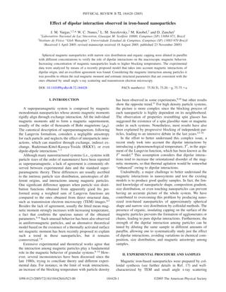
FIG. 1. A TEM image of the nanoparticle sample used in this
work. The insets show the SAXS curve of the same sample ͑the fit
is represented by the white line͒ and the distribution of sizes obtained from both techniques.
͑SAXS͒. The results of both analyses are shown in Fig. 1.
The TEM image shows spherical nanoparticles with mean
diameter, dav = 7.1 nm and very narrow size distribution ͑
= 0.08͒. This result is corroborated by the SAXS data of the
same sample, which shows an oscillatory behavior typical of
narrow size distribution spherical particles ͑inset of Fig. 1͒.
SAXS data treatment was done using the GNOM program,18
for which a sphere distribution was assumed. The SAXS
analysis gave dav = 7.3 nm, similar to TEM, but a larger size
distribution ͑ = 0.17͒. The distribution of particle sizes obtained by TEM and SAXS are shown in the inset of Fig. 1. It
is important to point out that the difference found between
the size distributions obtained by TEM and SAXS is not
surprising for this kind of sample. It is known that during the
solvent evaporation on the TEM grid the nanoparticles selfassemble forming large ordered regions of particles of similar sizes, excluding the smaller ones to the edges.19 This may
underestimate the TEM size distribution width. In this work
we have used the size distribution obtained by SAXS since it
gives an average signal and we consider that it better describes the actual system. In the following analysis, the
SAXS distribution of particle sizes has been converted to a
volume distribution and fitted with a Gaussian function,
given a volume distribution of V = 0.38.
The as-synthesized nanoparticles are mainly composed by
amorphous Fe and capped by oleyl-sarcosine molecules,
which avoid agglomeration. The colloidal solution can be
precipitated using methanol or ethanol and easily redispersed
in toluene or Decalin. The slow oxidation process leads to a
disordered Fe oxide, whose majority magnetic phase locally
resembles magnetite ͑Fe3O4͒, as identified by Mössbauer
spectroscopy.17 To evaluate the dipolar magnetic interaction
FIG. 2. The ZFC-FC curves as a function of nanoparticle concentration ͑H = 20 Oe͒. Note that the blocking temperature clearly
shifts to higher values when nanoparticle concentration increases.
The irreversibility region in the FC curves shows qualitatively the
increase of the dipolar interaction for higher nanoparticle
concentration.
in this system, some quantity of the same batch of the colloidal solution was precipitated ͑powder sample͒ or diluted
in paraffin, in different concentrations. This strategy was
adopted to minimize little variations that may occur when
using different batches of samples or due to the oxidation
process. The dilutions used in this work were 0.05, 0.5, 5,
and 45 % mass of colloid/mass of paraffin, hereinafter
named C005, C05, C5, and C45, respectively. However, it is
important to point out that the absolute values are just indicative of the degree of concentration due to the intrinsic large
errors in the determination of the actual magnetic nanoparticle core mass.
Zero-field-cooled ͑ZFC͒ and field-cooled ͑FC͒ magnetization and magnetization vs applied field ͑M vs H͒ measurements ͑magnetization loops͒ were performed in a commercial superconducting quantum interference device ͑SQUID͒
magnetometer ͑quantum design MPMS XL7͒. The diamagnetic contribution of the paraffin was subtracted from the
magnetization data and the results were presented in the reduced form for all samples, i.e., M / M S vs H, to avoid misleading results due to the uncertainties in the nanoparticle
mass determination.
III. RESULTS AND DISCUSSION
A. Magnetic properties
ZFC and FC curves as functions of particle concentration
are shown in Fig. 2 ͑H = 20 Oe͒. As can be clearly seen, for
increasing particle concentration the splitting points between
ZFC and FC curves as well as the maxima of the ZFC curves
shift to higher temperatures, indicating an increase in the
blocking temperature, TB.20 A similar trend was previously
observed by Dormann et al., Zysler et al.,21,22 and in Monte
Carlo simulations,23,24 for example. Such results qualitatively
184428-2
3. PHYSICAL REVIEW B 72, 184428 ͑2005͒
EFFECT OF DIPOLAR INTERACTION OBSERVED IN…
agree with the Dormann-Bessais-Fiorani model.9 Also, the
FC magnetization curvature in the irreversibility region ͑below blocking temperature͒ qualitatively marks the strength of
interparticle interaction, diminishing its relative height with
respect to the maximum of the ZFC curve as the concentration increases. It is worth mentioning that the overall shape
of the ZFC curves for all samples is similar, indicating that
no percolation occurs among particles, so reassuring that the
magnetic properties can be, in principle, described in the
framework of the superparamagnetic model. In some systems composed by nanoparticles, when the volume concentration of the magnetic element reaches 17–25 %, a clear
distinctive shape of the ZFC curve appears due to direct contact among magnetic nanoparticles.25,26
It is known that the ZFC curve is sensitive to the distribution of activation energy ͑25 kTB͒ that can be easily calculated considering a system of noninteracting particles with
x volume concentration of particles.20 For a single particle of
volume, V, the magnetization, M, under low magnetic field,
H, is expressed as M = ͑M core͒2 VH / kT in the superparamagS
netic region ͑T Ͼ TB͒, and M = ͑M core͒2 H / 3 K in the blocked
S
region ͑T Ͻ TB͒, respectively ͑T is the system temperature,
M core is the saturation magnetization of the nanoparticle
S
magnetic core, k is the Boltzmann constant, and K is the
anisotropy constant͒. Therefore, for a noninteracting fine particle system the total magnetization can be written as27
M ZFC͑H,T͒ M coreH
= S
MS
3K
+
͵
͵
ϱ
f͑V͒dV
Vb͑T͒
M coreH
S
3kT
Vb͑T͒
Vf͑V͒dV,
͑1͒
0
where Vb͑T͒ = 25kT / K, and f͑V͒ is the particle volume distribution, and M S is the sample saturation magnetization, ͑x
is the magnetic core volume fraction͒. The first term in Eq.
͑1͒ describes the contribution of the particles in the blocked
state. Its relative contribution drops with increasing temperature, as the number of the blocked particles decreases. The
f͑V͒ can be related to the distribution of blocking temperature by the linear expression 25kTB = KV. Therefore, one can
obtain K by fitting the ZFC curves using V = 0.38 obtained
by SAXS, and the M S value obtained from the M vs H measured at low temperatures ͑keeping M core and K as free fitting
S
parameters͒. Figure 3 shows the reduced curve for the most
diluted sample ͑C005͒ and the corresponding fit. From this
analysis, K = 3.6ϫ 105 erg/ cm3 and M core = 490 emu/ cm3. As
S
can be seen in Fig. 3, the superparamagnetic model is a good
approach to describe the C005 sample behavior, suggesting
that the possibility of particles agglomeration is not significant in that sample. In addition, this result confirms the morphological information derived from SAXS.
The coercive field, HC, obtained from the M / M S vs H
curves measured at different temperatures is shown in Fig. 4
͑at temperatures below the blocking one͒. The coercive field
temperature behavior of systems of identical noninteracting
particles with random anisotropy axes follows the wellknown relation,28
FIG. 3. The zero-field cooled curve of a C005 sample measured
with H = 20 Oe. The line is the best fit of Eq. ͑1͒ to the experimental
data ͑symbol͒ using the SAXS distribution and M core and K as free
S
parameters.
Hc = 0.96
K
͓1 − ͑T/TB͒1/2͔.
M core
S
͑2͒
It can be inferred from Fig. 4 that the HC behavior of the
samples C5 and C45 can be described by Eq. ͑2͒ at least in
the low temperature range, giving K / M core = 670 Oe and 636
S
Oe, respectively. This simple approximation, however, does
not hold reasonably for the powder sample. The decrease of
the HC value for sample C45 compared to C5 is in agreement
with the demagnetizing role played by the dipolar interaction
as simulated by Kechrakos and Trohidou.29 The Hc vs T
trends also confirm that the only parameter change in our
samples is the particle concentration. Using the K value obtained from the ZFC analysis of C005 sample, we find
FIG. 4. HC vs T0.5 obtained for the C5, C45, and powder
samples. Similar behavior of samples C5 and C45 can be seen. In
addition, these samples present a linear dependence with T0.5 in the
low temperature range. The lines serve as a guide to the eyes.
184428-3
4. PHYSICAL REVIEW B 72, 184428 ͑2005͒
VARGAS et al.
is not simply a fitting parameter. It can be related to the rms
dipolar energy D,
D = kT* = ␣ 2/D3 ,
͑4͒
where ␣ is a constant ͑derived from the sum of all dipolar
energy contributions͒, and D is the average interparticle
distance.4 This is the main assumption of the T* model that
considers that a dipolar field exerts a disordering and random
torque to the magnetic moments of the particles, “decreasing” the ordering effect played by the applied magnetic field
͑similar to the effect of temperature͒.
Using the condition ND3 = 1 and M S = N, T* can be calculated as
FIG. 5. The M vs H curves of C5, C45 and powder samples
pointing out the effect of the dipolar interaction. The inset shows
the C5 data as a function of temperature and the corresponding fits
using the conventional superparamagnetic model showing a nice
agreement but spurious values ͑these values correspond to the a
in the T* model͒.
M core = 537 emu/ cm3 and M core = 564 emu/ cm3 for samples
S
S
C5 and C45. Considering the approximations involved in
both fits, the results are in very good agreement with the
ZFC analysis.
M / M S vs H curves have been measured at several temperatures for all samples. The loops of sample C005 and C05
were strongly influenced by paraffin diamagnetism, which
screens the high-field region of the measurements, and therefore those results will not be considered in the following
analysis. Figure 5 shows the M / M S vs H of C5, C45, and
powder samples measured at 300 K showing the effect of
dilution. The inset shows the evolution of M / M S vs H of C5
as a function of temperature. It is important to mention that
the universal curve M / M S vs H / T, expected in a canonical
superparamagnetic system when plotting M vs H curves
taken at different temperatures, cannot be obtained.30 This
lack of agreement is more pronounced for the powder
sample, as expected due to stronger interparticle interactions.
T* =
a =
͵ ͩ
ϱ
0
L
ͪ
H
f͑͒d ,
k͑T + T*͒
1
͑3͒
where N is the number of particles per unit volume, f͑͒ is
the distribution of magnetic moments that is determined
from the experimental volume distribution ͑ = M coreV͒, and
S
L is the Langevin function. It is important to remark that T*
ͩ ͪ
*.
Na = 1 +
T
1+
T
T*
N,
T
͑6͒
and, as a consequence,
͵ ͩ ͪ
ϱ
M͑H,T͒ = Na
aL
0
aH
f͑a͒da .
kT
͑7͒
The only two fitting parameters are Na and a for each
temperature and Na is assumed to be independent of temperature, since f͑ua͒ was obtained from SAXS. In this work
we used the reduced form of Eq. ͑7͒, reducing the fitting
parameters to a single parameter, a, for each temperature:
͵ ͩ ͪ
͵
ϱ
M͑H,T͒
=
MS
To study in more detail the effect of interparticle interactions as function of particle concentration, we have employed the T* model.4 In such a model, the effect of the
dipolar interaction is introduced by means of a fictitious temperature, T*, which is added to the actual temperature T in
the denominator of the Langevin function argument. This
phenomenological theory can be used to relate the experimental magnetization M of a set of interacting nanoparticles
to their actual magnetic moment ,
͑5͒
Equation ͑3͒ can be rewritten as a weighted sum of standard Langevin functions, but considering instead an apparent
magnetic moment a and an apparent particle density, Na,
given by,4
B. Influence of the dipolar interaction
M͑H,T͒ = N
␣ 2 ␣
␣ M2
S
2
.
3 = N =
kD
k
k N
aL
0
ϱ
aH
f͑a͒da
kT
.
͑8͒
a f͑a͒da
0
The M / M S vs H curves fits for each temperature were
very good in all cases ͑see inset in Fig. 5 for the analysis of
C5 sample͒ and the inset of Fig. 6 shows the a as a function
of temperature for the three considered samples. It can be
inferred from Fig. 6 an increase of a with the temperature
up to a maximum value, depending on sample concentration.
Since all samples have the same magnetic anisotropy, this
reinforces the hypothesis of the existence of a strict relationship between the dipolar interaction and the anomalous thermal behavior of a, commonly observed in single domain
particle systems.4
The only required parameter to calculate the real magnetic
moment from a is T* ͓see Eq. ͑6͔͒. The T* can be derived
from the low-field susceptibility of an interacting superparamagnetic system within the framework of this model,
184428-4
5. PHYSICAL REVIEW B 72, 184428 ͑2005͒
EFFECT OF DIPOLAR INTERACTION OBSERVED IN…
FIG. 6. a and values as a function of temperature for C5 ͑
taken constant͒. The inset shows the a values for the three
samples.
=
N2
,
3k͑T + T*͒
͑9͒
which, for a system with size distribution, can be expressed
as4
ͩ ͪ
T
= 3kN
+ 3␣ = AT + C,
M2
S
͑10͒
where = ͗2͘ / ͗͘2 = ͗2͘ / ͗a͘2, the brackets indicating the
a
average over the values of the distribution of magnetic moments ͑see details in Ref. 4͒. T* can now be readily obtained
from the ratio C / A ͓͑see Eqs. ͑5͒ and ͑10͔͒. The curve
/ vs T can be independently obtained from different
routes, such as the high-temperature region of the ZFC-FC
curves, i.e., above blocking temperature, or from the lowfield region of the anhysteretic curves ͑average of two
branches of a hysteresis loop31͒. In the present case, the ͑T͒
values were obtained of the linear region of the anhysteretic
magnetization curves. The fit was performed in the linear
region of the normalized form of Eq. ͑10͒, M S / vs T, using M S ͑in emu͒ at 20 K, and the results are presented in
Table I and Fig. 7. It is interesting to note in Fig. 7 that the
angular coefficient, M SA, which is equal to 3k / , is similar
to the three samples as it should be expected since the only
variable parameter among samples is the concentration. It is
important to point out, however, that T* may be underestimated by taking the normalization, M S, at 20 K, but the
TABLE I. The values of M SA and M SC derived from the fit of
M S / vs T using Eq. ͑10͒ and the resulting values of T*. The
value obtained from the SAXS volume distribution was 1.13.
FIG. 7. The M S / vs T graphic obtained from the linear region
of the magnetization curves ͑magnetization under low field H͒ for
the three samples. The solid lines are the best fits done to derive the
T* values ͑see the text͒.
correct trend among samples is still obtained.
Figure 6 shows the real magnetic moment obtained
from a and T* ͑considering M S constant with temperature͒.
To corroborate the analysis, the temperature dependence of
the a calculated by using the T* and are shown by lines in
the inset of Fig. 6, showing a good agreement with the results obtained via the fit of M / H vs H curves at different
temperatures.
We have also tested different approaches to fit the
M / M S x H curves, for example, considering T* and as
fitting parameters, where curves taken at different temperatures are fitted simultaneously. The results and goodness of
the fits were similar to the previous case. We have also tested
to leave the moment distribution width as a free parameter,
and it converged to the value derived from the SAXS analysis for all samples, further validating the analysis.
It is worth emphasizing that good fits using a properly
weighted set of Langevin functions are not surprising, but
often the obtained size distribution parameters are quite different from those obtained from direct structural
measurements.4–6,32 However, considering the T* model applied in the present work, the fitting parameters agree rather
well with structural data. One can estimate the mean magnetic moment, ͗͘ = M coreV, by considering spherical parS
ticles, dav = 7.3 nm, and M S = 537 emu/ cm3 ͑calculated from
the coercivity measurements for sample C5͒. This procedure
leads to a value of the magnetic moment, ͗͘ = 11802 B,
which is rather close to the values obtained from the T*
model.
Sample
M SA
M SC
T* ͑K͒
IV. CONCLUSION
C5
C45
Powder
3.3
3.5
3.2
173
266
622
51.7
76.1
196.1
In this work, spherical magnetic nanoparticles with narrow size distribution and organic capping were diluted in
paraffin with different concentrations to tune interparticle
dipole-dipole interactions. We clearly demonstrated that a
184428-5
6. PHYSICAL REVIEW B 72, 184428 ͑2005͒
VARGAS et al.
shift of the blocking temperature with increasing concentrations is observed when solely dipolar interactions are
strengthened. Morover, to the best of our knowledge, this is
the first experimental test of the T* model using a wellbehaved system composed by truly isolated spherical nanoparticles with narrow size distribution. Using this model, we
were able to derive the correct trends among samples and the
real magnetic moment, which was in good agreement with
ZFC-FC and Hc analysis. Also, different fit routes were
tested, and all of them converged to very similar values, very
close to those obtained from structural data. Such data and
their analysis point to an adequacy of such a phenomenologi-
*Present address: Centro Atómico Bariloche, Avenue Bustillo 9.
500͑R8402AGP͒ San Carlos de Bariloche ͑RN͒, Argentina.
1 L. Néel, Ann. Geophys. ͑C.N.R.S.͒ 5, 99 ͑1949͒.
2
X. Battle and A. Labarta, J. Phys. D 35, R15 ͑2002͒.
3 R. Skomski, J. Phys.: Condens. Matter 15, R841 ͑2003͒.
4
P. Allia, M. Coisson, P. Tiberto, F. Vinai, M. Knobel, M. A. Novak, and W. C. Nunes, Phys. Rev. B 64, 144420 ͑2001͒.
5
A. L. Brandl, J. C. Denardin, L. M. Socolovsky, M. Knobel, and
P. Allia, J. Magn. Magn. Mater. 272-276, 1526 ͑2004͒.
6 H. Mamiya, I. Nakatani, T. Furubayashi, and M. Ohnuma, Trans.
Magn. Soc. Jpn. 2, 36 ͑2002͒.
7 S. Mørup and C. Frandsen, Phys. Rev. Lett. 92, 217201 ͑2004͒;N.
J. O. Silva, L. D. Carlos, and V. S. Amaral, ibid. 94, 039707
͑2005͒;S. Morup and C. Frandsen, ibid. 94, 039708 ͑2005͒;A.
H. MacDonald and C. M. Canali, ibid. 94, 089701 ͑2005͒;S.
Morup and C. Frandsen, ibid. 94, 089702 ͑2005͒.
8 M. Knobel, W. C. Nunes, A. L. Brandl, J. M. Vargas, L. M.
Socolovsky, and D. Zanchet, Physica B 354, 80 ͑2004͒.
9 J. L. Dormann, L. Bessais, and D. Fiorani, J. Phys. C 21, 2015
͑1988͒;J. L. Dormann, D. Fiorani, and E. Tronc, J. Magn. Magn.
Mater. 202, 251 ͑1999͒.
10 W. Luo, S. R. Nagel, T. F. Rosenbaum, and R. E. Rosensweig,
Phys. Rev. Lett. 67, 2721 ͑1991͒.
11 S. Mørup and E. Tronc, Phys. Rev. Lett. 72, 3278 ͑1994͒.
12 Y. Sun, M. B. Salamon, K. Garnier, and R. S. Averback, Phys.
Rev. Lett. 91, 167206 ͑2003͒;M. Sasaki, P. E. Jönsson, H.
Takayama, and P. Nordblad, ibid. 93, 139701 ͑2004͒.
13
M. F. Hansen et al., J. Phys.: Condens. Matter 14, 4901 ͑2002͒.
14 W. Kleemann, O. Petracic, C. Binek, G. N. Kakazei, Y. G.
Pogorelov, J. B. Sousa, O. S. Cardos, and P. P. Freitas, Phys.
Rev. B 63, 134423 ͑2001͒.
15 E. P. Wohlfarth, Physica B & C 86, 852 ͑1977͒.
16
S. Chakraverty, M. Bandyopadhyay, S. Chatterjee, S. Dattagupta,
cal model to explain the trends of the intricate macroscopic
magnetic behavior of a superparamagnetic system with the
presence of dipolar interactions among magnetic particles.
However, further analysis should be carried out to further
corroborate quantitatively the results derived from this
model.
ACKNOWLEDGMENT
Brazilian funding agencies FAPESP, CAPES, CNPq, and
Brazilian Synchrotron Light Laboratory ͑SAXS beamline
and LME͒ are acknowledged for their support.
A. Frydman, S. Sengupta, and P. A. Sreeram, Phys. Rev. B 71,
054401 ͑2005͒.
17 J. M. Vargas, L. M. Socolovsky, G. F. Goya, M. Knobel, and D.
Zanchet, IEEE Trans. Magn. 39, 2681 ͑2003͒.
18 D. I. Svergun, J. Appl. Crystallogr. 25, 495 ͑1992͒.
19
P. C. Ohara, D. V. Leff, J. R. Heath, and W. M. Gelbart, Phys.
Rev. Lett. 75, 3466 ͑1995͒.
20
J. C. Denardin, A. L. Brandl, M. Knobel, P. Panissod, A. B.
Pakhomov, H. Liu, and X. X. Zhang, Phys. Rev. B 65, 64422
͑2002͒.
21 J. L. Dormann, D. Fiorani, and E. Tronc, Adv. Chem. Phys., 98,
283 ͑1997͒.
22
R. D. Zysler, C. A. Ramos, E. De Biasi, H. Romero, A. Ortega,
and D. Fiorani, J. Magn. Magn. Mater. 221, 37 ͑2000͒.
23
J. García-Otero, M. Porto, J. Rivas, and A. Bunde, Phys. Rev.
Lett. 84, 167 ͑2000͒.
24 M. Bahiana, J. P. Pereira Nunes, D. Altbir, P. Vargas, and M.
Knobel, J. Magn. Magn. Mater. 281, 372 ͑2004͒.
25 B. V. B. Sarkissian, J. Phys.: Condens. Matter 208, 2191 ͑1981͒.
26
L. M. Socolovsky, F. H. Sánchez, and P. H. Shingu, Hyperfine
Interact. 133, 47 ͑2001͒.
27 T. Bitoh, K. Ohba, M. Takamatsu, T. Shirane, and S. Chikazawa,
J. Phys. Soc. Jpn. 64, 1305 ͑1995͒.
28 E. F. Kneller and F. E. Luborsky, J. Appl. Phys. 34, 656 ͑1963͒.
29 D. Kechrakos and K. N. Trohidou, Phys. Rev. B 58, 12169
͑1998͒.
30 I. S. Jacobs and C. P. Bean, in Magnetism, edited by G. T. Rado
and H. Suhl ͑New York, Academic Press, 1963͒, Vol. III,
pp.271-350.
31 P. Allia, M. Coisson, M. Knobel, P. Tiberto, and F. Vinai, Phys.
Rev. B 60, 17 12207 ͑1999͒.
32 Q. A. Pankhurst, D. H. Ucko, L. Fernández Barquín, and R.
García Calderón, J. Magn. Magn. Mater. 266, 131 ͑2003͒.
184428-6