1) The document discusses directional derivatives and the gradient of functions of several variables. It defines the directional derivative Duf(c) as the slope of the function f in the direction of the unit vector u at the point c. 2) It shows that the partial derivatives of f can be computed by treating all but one variable as a constant. The gradient of f is defined as the vector of its partial derivatives. 3) It derives an expression for the directional derivative Duf(c) in terms of the partial derivatives of f and the components of the unit vector u, showing the relationship between directional derivatives and the gradient.

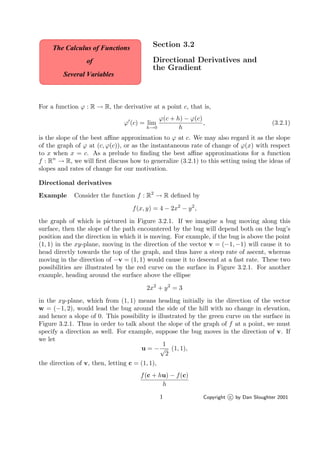
1. Several Variables
The Calculus of Functions
of
Section 3.2
Directional Derivatives and
the Gradient
For a function ϕ : R → R, the derivative at a point c, that is,
ϕ (c) = lim
h→0
ϕ(c + h) − ϕ(c)
h
, (3.2.1)
is the slope of the best affine approximation to ϕ at c. We may also regard it as the slope
of the graph of ϕ at (c, ϕ(c)), or as the instantaneous rate of change of ϕ(x) with respect
to x when x = c. As a prelude to finding the best affine approximations for a function
f : Rn
→ R, we will first discuss how to generalize (3.2.1) to this setting using the ideas of
slopes and rates of change for our motivation.
Directional derivatives
Example Consider the function f : R2
→ R defined by
f(x, y) = 4 − 2x2
− y2
,
the graph of which is pictured in Figure 3.2.1. If we imagine a bug moving along this
surface, then the slope of the path encountered by the bug will depend both on the bug’s
position and the direction in which it is moving. For example, if the bug is above the point
(1, 1) in the xy-plane, moving in the direction of the vector v = (−1, −1) will cause it to
head directly towards the top of the graph, and thus have a steep rate of ascent, whereas
moving in the direction of −v = (1, 1) would cause it to descend at a fast rate. These two
possibilities are illustrated by the red curve on the surface in Figure 3.2.1. For another
example, heading around the surface above the ellipse
2x2
+ y2
= 3
in the xy-plane, which from (1, 1) means heading initially in the direction of the vector
w = (−1, 2), would lead the bug around the side of the hill with no change in elevation,
and hence a slope of 0. This possibility is illustrated by the green curve on the surface in
Figure 3.2.1. Thus in order to talk about the slope of the graph of f at a point, we must
specify a direction as well. For example, suppose the bug moves in the direction of v. If
we let
u = −
1
√
2
(1, 1),
the direction of v, then, letting c = (1, 1),
f(c + hu) − f(c)
h
1 Copyright c by Dan Sloughter 2001

2. 2 Directional Derivatives and the Gradient Section 3.2
-2
-1
0
1
2 x
-2 -1 0 1 2
y
-2
0
2
4
z
-2
-1
0
1
2 x
-2 -1 0 1 2
y
Figure 3.2.1 Graph of f(x) = 4 − 2x2
− y2
would, for any h > 0, represent an approximation to the slope of the graph of f at (1, 1)
in the direction of u. As in single-variable calculus, we should expect that taking the limit
as h approaches 0 should give us the exact slope at (1, 1) in the direction of u. Now
f(c + hu) − f(c) = f 1 −
h
√
2
, 1 −
h
√
2
− f(1, 1)
= 4 − 2 1 −
h
√
2
2
− 1 −
h
√
2
2
− 1
= 3 − 3 1 −
√
2h +
h2
2
= 3
√
2h −
3h2
2
= h 3
√
2 −
3h
2
,
so
lim
h→0
f(c + hu) − f(c)
h
= lim
h→0
3
√
2 −
3h
2
= 3
√
2.
Hence the graph of f has a slope of 3
√
2 if we start above (1, 1) and head in the direction
of u; similar computations would show that the slope in the direction of −u is −3
√
2 and
the slope in the direction of

3. Section 3.2 Directional Derivatives and the Gradient 3
w
w
=
1
√
5
(−1, 2)
is 0.
Definition Suppose f : Rn
→ R is defined on an open ball about a point c. Given a
unit vector u, we call
Duf(c) = lim
h→0
f(c + hu) − f(c)
h
, (3.2.2)
provided the limit exists, the directional derivative of f in the direction of u at c.
Example From our work above, if f(x, y) = 4 − 2x2
− y2
and
u = −
1
√
2
(1, 1),
then Duf(1, 1) = 3
√
2.
Directional derivatives in the direction of the standard basis vectors will be of special
importance.
Definition Suppose f : Rn
→ R is defined on an open ball about a point c. If we
consider f as a function of x = (x1, x2, . . . , xn) and let ek be the kth standard basis
vector, k = 1, 2, . . . , n, then we call Dek
f(c), if it exists, the partial derivative of f with
respect to xk at c.
Notations for the partial derivative of f with respect to xk at an arbitrary point
x = (x1, x2, . . . , xn) include Dxk
f(x1, x2, . . . , xn), fxk
(x1, x2, . . . , xn), and
∂
∂xk
f(x1, x2, . . . , xn).
Now suppose f : Rn
→ R and, for fixed x = (x1, x2, . . . , xn), define g : R → R by
g(t) = f(t, x2, . . . , xn).
Then
fx1
(x1, x2, . . . , xn) = lim
h→0
f((x1, x2, . . . , xn) + he1) − f(x1, x2, . . . , xn)
h
= lim
h→0
f((x1, x2, . . . , xn) + (h, 0, . . . , 0)) − f(x1, x2, . . . , xn)
h
= lim
h→0
f(x1 + h, x2, . . . , xn) − f(x1, x2, . . . , xn)
h
= lim
h→0
g(x1 + h) − g(x1)
h
= g (x1).
(3.2.3)

4. 4 Directional Derivatives and the Gradient Section 3.2
In other words, we may compute the partial derivative fx1 (x1, x2, . . . , xn) by treating
x2, x3, . . . , xn as constants and differentiating with respect to x1 as we would in single-
variable calculus. The same statement holds for any coordinate: To find the partial
derivative with respect to xk, treat the other coordinates as constants and differentiate
as if the function depended only on xk.
Example If f : R2
→ R is defined by
f(x, y) = 3x2
− 4xy2
,
then, treating y as a constant and differentiating with respect to x,
fx(x, y) = 6x − 4y2
and, treating x as a constant and differentiating with respect to y,
fy(x, y) = −8xy.
Example If f : R4
→ R is defined by
f(w, x, y, z) = − log(w2
+ x2
+ y2
+ z2
),
then
∂
∂w
f(w, z, y, z) = −
2w
w2 + x2 + y2 + z2
,
∂
∂x
f(w, z, y, z) = −
2x
w2 + x2 + y2 + z2
,
∂
∂y
f(w, z, y, z) = −
2y
w2 + x2 + y2 + z2
,
and
∂
∂z
f(w, z, y, z) = −
2z
w2 + x2 + y2 + z2
.
Example Suppose g : R2
→ R is defined by
g(x, y) =



xy
x2 + y2
, if (x, y) = (0, 0),
0, if (x, y) = (0, 0).
We saw in Section 3.1 that lim
(x,y)→(0,0)
g(x, y) does not exist; in particular, g is not continuous
at (0, 0). However,
∂
∂x
g(0, 0) = lim
h→0
g((0, 0) + h(1, 0)) − g(0, 0)
h
= lim
h→0
g(h, 0)
h
= lim
h→0
0
h
= 0

5. Section 3.2 Directional Derivatives and the Gradient 5
and
∂
∂y
g(0, 0) = lim
h→0
g((0, 0) + h(0, 1)) − g(0, 0)
h
= lim
h→0
g(0, h)
h
= lim
h→0
0
h
= 0.
This shows that it is possible for a function to have partial derivatives at a point without
being continuous at that point. However, we shall see in Section 3.3 that this function is
not differentiable at (0, 0); that is, f does not have a best affine approximation at (0, 0).
The gradient
Definition Suppose f : Rn
→ R is defined on an open ball containing the point c and
∂
∂xk
f(c) exists for k = 1, 2, . . . , n. We call the vector
f(c) =
∂
∂x1
f(c),
∂
∂x2
f(c), . . . ,
∂
∂xn
f(c) (3.2.4)
the gradient of f at c.
Example If f : R2
→ R is defined by
f(x, y) = 3x2
− 4xy2
,
then
f(x, y) = (6x − 4y2
, −8xy).
Thus, for example, f(2, −1) = (8, 16).
Example If f : R4
→ R is defined by
f(w, x, y, z) = − log(w2
+ x2
+ y2
+ z2
),
then
f(w, x, y, z) = −
2
w2 + x2 + y2 + z2
(w, x, y, z).
Thus, for example,
f(1, 2, 2, 1) = −
1
5
(1, 2, 2, 1).
Notice that if f : Rn
→ R, then f : Rn
→ Rn
; that is, we may view the gradient as a
function which takes an n-dimensional vector for input and returns another n-dimensional
vector. We call a function of this type a vector field.
Definition We say a function f : Rn
→ R is C1
on an open set U if f is continuous on
U and, for k = 1, 2, . . . , n, ∂f
∂xk
is continuous on U.

6. 6 Directional Derivatives and the Gradient Section 3.2
Now suppose f : R2
→ R is C1
on some open ball containing the point c = (c1, c2). Let
u = (u1, u2) be a unit vector and suppose we wish to compute the directional derivative
Duf(c). From the definition, we have
Duf(c) = lim
h→0
f(c + hu) − f(c)
h
= lim
h→0
f(c1 + hu1, c2 + hu2) − f(c1, c2)
h
= lim
h→0
f(c1 + hu1, c2 + hu2) − f(c1 + hu1, c2) + f(c1 + hu1, c2) − f(c1, c2)
h
= lim
h→0
f(c1 + hu1, c2 + hu2) − f(c1 + hu1, c2)
h
+
f(c1 + hu1, c2) − f(c1, c2)
h
.
For a fixed value of h = 0, define ϕ : R → R by
ϕ(t) = f(c1 + hu1, c2 + t). (3.2.5)
Note that ϕ is differentiable with
ϕ (t) = lim
s→0
ϕ(t + s) − ϕ(t)
s
= lim
s→0
f(c1 + hu1, c2 + t + s) − f(c1 + hu1, c2 + t)
s
=
∂
∂y
f(c1 + hu1, c2 + t).
(3.2.6)
Hence if we define α : R → R by
α(t) = ϕ(u2t) = f(c1 + hu1, c2 + tu2), (3.2.7)
then α is differentiable with
α (t) = u2ϕ (u2t) = u2
∂
∂y
f(c1 + hu1, c2 + tu2). (3.2.8)
By the Mean Value Theorem from single-variable calculus, there exists a number a between
0 and h such that
α(h) − α(0)
h
= α (a). (3.2.9)
Putting (3.2.7) and (3.2.8) into (3.2.9), we have
f(c1 + hu1, c2 + hu2) − f(c1 + hu2, c2)
h
= u2
∂
∂y
f(c1 + hu1, c2 + au2). (3.2.10)
Similarly, if we define β : R → R by
β(t) = f(c1 + tu1, c2), (3.2.11)

7. Section 3.2 Directional Derivatives and the Gradient 7
then β is differentiable,
β (t) = u1
∂
∂x
f(c1 + tu1, c2), (3.2.12)
and, using the Mean Value Theorem again, there exists a number b between 0 and h such
that
f(c1 + hu1, c2) − f(c1, c2)
h
=
β(h) − β(0)
h
= β (b) = u1
∂
∂x
f(c1 + bu1, c2). (3.2.13)
Putting (3.2.10) and (3.2.13) into our expression for Duf(c) above, we have
Duf(c) = lim
h→0
u2
∂
∂y
f(c1 + hu1, c2 + au2) + u1
∂
∂x
f(c1 + bu1, c2) . (3.2.14)
Now both a and b approach 0 as h approaches 0 and both ∂f
∂x and ∂f
∂y are assumed to be
continuous, so evaluating the limit in (3.2.14) gives us
Duf(c) = u2
∂
∂y
f(c1, c2) + u1
∂
∂x
f(c1, c2) = f(c) · u. (3.2.15)
A straightforward generalization of (3.2.15) to the case of a function f : Rn
→ R gives
us the following theorem.
Theorem Suppose f : Rn
→ R is C1
on an open ball containing the point c. Then for
any unit vector u, Duf(c) exists and
Duf(c) = f(c) · u. (3.2.16)
Example If f : R2
→ R is defined by
f(x, y) = 4 − 2x2
− y2
,
then
f(x, y) = (−4x, −2y).
If
u = −
1
√
2
(1, 1),
then
Duf(1, 1) = f(1, 1) · u = (−4, −2) · −
1
√
2
(1, 1) =
6
√
2
= 3
√
2,
as we saw in this first example of this section. Note also that
D−uf(1, 1) = f(1, 1) · (−u) = (−4, −2) ·
1
√
2
(1, 1) = −
6
√
2
= −3
√
2

8. 8 Directional Derivatives and the Gradient Section 3.2
and, if
w =
1
√
5
(−1, 2),
Dwf(1, 1) = f(1, 1) · (w) = (−4, −2) ·
1
√
5
(−1, 2) = 0,
as claimed earlier.
Example Suppose the temperature at a point in a metal cube is given by
T(x, y, z) = 80 − 20xe− 1
20 (x2
+y2
+z2
)
,
where the center of the cube is taken to be at (0, 0, 0). Then we have
∂
∂x
T(x, y, z) = 2x2
e− 1
20 (x2
+y2
+z2
)
− 20e− 1
20 (x2
+y2
+z2
)
,
∂
∂y
T(x, y, z) = 2xye− 1
20 (x2
+y2
+z2
)
,
and
∂
∂z
T(x, y, z) = 2xze− 1
20 (x2
+y2
+z2
)
,
so
T(x, y, z) = e− 1
20 (x2
+y2
+z2
)
(2x2
− 20, 2xy, 2xz).
Hence, for example, the rate of change of temperature at the origin in the direction of the
unit vector
u =
1
√
3
(1, −1, 1)
is
DuT(0, 0, 0) = T(0, 0, 0) · u = (−20, 0, 0) ·
1
√
3
(1, −1, 1) = −
20
√
3
.
An application of the Cauchy-Schwarz inequality to (3.2.16) shows us that
|Duf(c)| = | f(c) · u| ≤ f(c) u = f(c) . (3.2.17)
Thus the magnitude of the rate of change of f in any direction at a given point never
exceeds the length of the gradient vector at that point. Moreover, in our discussion of
the Cauchy-Schwarz inequality we saw that we have equality in (3.2.17) if and only if u is
parallel to f(c). Indeed, supposing f(c) = 0, when
u =
f(c)
f(c)
,

9. Section 3.2 Directional Derivatives and the Gradient 9
we have
Duf(c) = f(c) · u =
f(c) · f(c)
f(c)
=
f(c) 2
f(c)
= f(c) (3.2.18)
and
D−uf(c) = − f(c) . (3.2.19)
Hence we have the following result.
Proposition Suppose f : Rn
→ R is C1
on an open ball containing the point c. Then
Duf(c) has a maximum value of f(c) when u is the direction of f(c) and a minimum
value of − f(c) when u is the direction of − f(c).
In other words, the gradient vector points in the direction of the maximum rate of
increase of the function and the negative of the gradient vector points in the direction of
the maximum rate of decrease of the function. Moreover, the length of the gradient vector
tells us the rate of increase in the direction of maximum increase and its negative tells us
the rate of decrease in the direction of maximum decrease.
Example As we saw above, if f : R2
→ R is defined by
f(x, y) = 4 − 2x2
− y2
,
then
f(x, y, ) = (−4x, −2y).
Thus f(1, 1) = (−4, −2). Hence if a bug standing above (1, 1) on the graph of f wants
to head in the direction of most rapid ascent, it should move in the direction of the unit
vector
u =
f(1, 1)
f(1, 1)
= −
1
√
5
(2, 1).
If the bug wants to head in the direction of most rapid descent, it should move in the
direction of the unit vector
−u =
1
√
5
(2, 1).
Moreover,
Duf(1, 1) = f(1, 1) =
√
20
and
D−uf(1, 1) = − f(1, 1) = −
√
20.
Figure 3.2.2 shows scaled values of f(x, y) plotted for a grid of points (x, y). The vec-
tors are scaled so that they fit in the plot, without overlap, yet still show their relative
magnitudes. This is another good geometric way to view the behavior of the function.
Supposing our bug were placed on the side of the graph above (1, 1) and that it headed up
the hill in such a manner that it always chose the direction of steepest ascent, we can see
that it would head more quickly toward the y-axis than toward the x-axis. More explicitly,

10. 10 Directional Derivatives and the Gradient Section 3.2
-1 -0.5 0.5 1 1.5 2
-1
-0.5
0.5
1
1.5
2
Figure 3.2.2 Scaled gradient vectors for f(x, y) = 4 − 2x2
− y2
if C is the shadow of the path of the bug in the xy-plane, then the slope of C at any point
(x, y) would be
dy
dx
=
−2y
−4x
=
y
2x
.
Hence
1
y
dy
dx
=
1
2x
.
If we integrate both sides of this equality, we have
1
y
dy
dx
dx =
1
2x
dx.
Thus
log |y| =
1
2
log |x| + c
for some constant c, from which we have
elog |y|
= e
1
2 log |x|+c
.
It follows that
y = k |x|,
where k = ±ec
. Since y = 1 when x = 1, k = 1 and we see that C is the graph of y =
√
x.
Figure 3.2.2 shows C along with the plot of the gradient vectors of f, while Figure 3.2.3
shows the actual path of the bug on the graph of f.

11. Section 3.2 Directional Derivatives and the Gradient 11
-2
-1
0
1
2 x
-2 -1 0 1 2
y
-2
0
2
4
z
-2
-1
0
1
2 x
-2 -1 0 1 2
y
Figure 3.2.3 Graph f(x, y) = 4 − 2x2
− y2
with path of most rapid ascent from (1, 1, 1)
Example For a two-dimensional version of the temperature example discussed above,
consider a metal plate heated so that its temperature at (x, y) is given by
T(x, y) = 80 − 20xe− 1
20 (x2
+y2
)
.
Then
T(x, y) = e− 1
20 (x2
+y2
)
(2x2
− 20, 2xy),
so, for example,
T(0, 0) = (−20, 0).
Thus at the origin the temperature is increasing most rapidly in the direction of u = (−1, 0)
and decreasing most rapidly in the direction of (1, 0). Moreover,
DuT(0, 0) = f(0, 0) = 20
and
D−uT(0, 0) = − f(0, 0) = 20.
Note that
D−uT(0, 0) =
∂
∂x
T(0, 0)
and
DuT(0, 0) = −
∂
∂x
T(0, 0).

12. 12 Directional Derivatives and the Gradient Section 3.2
-4 -2 2 4
-4
-2
2
4
Figure 3.2.4 Scaled gradient vectors for T(x, y) = 80 − 20xe− 1
20 (x2
+y2
)
Figure 3.2.4 is a plot of scaled gradient vectors for this temperature function. From the
plot it is easy to see which direction a bug placed on this metal plate would have to choose
in order to warm up as rapidly as possible. It should also be clear that the temperature
has a relative maximum around (−3, 0) and a relative minimum around (3, 0); these points
are, in fact, exactly (−
√
10, 0) and (
√
10, 0), the points where T(x, y) = (0, 0). We will
consider the problem of finding maximum and minimum values of functions of more than
one variable in Section 3.5.
Problems
1. Suppose f : R2
→ R is defined by
f(x, y) = 3x2
+ 2y2
.
Let
u =
1
√
5
(1, 2).
Find Duf(3, 1) directly from the definition (3.2.2).
2. For each of the following functions, find the partial derivatives with respect to each
variable.

13. Section 3.2 Directional Derivatives and the Gradient 13
(a) f(x, y) =
4x
x2 + y2
(b) g(x, y) = 4xy2
e−y2
(c) f(x, y, z) = 3x2
y3
z4
− 13x2
y (d) h(x, y, z) = 4xze
− 1
x2+y2+z2
(e) g(w, x, y, z) = sin( w2 + x2 + 2y2 + 3z2)
3. Find the gradient of each of the following functions.
(a) f(x, y, z) = x2 + y2 + z2 (b) g(x, y, z) =
1
x2 + y2 + z2
(c) f(w, x, y, z) = tan−1
(4w + 3x + 5y + z)
4. Find Duf(c) for each of the following.
(a) f(x, y) = 3x2
+ 5y2
, u =
1
√
13
(3, −2), c = (−2, 1)
(b) f(x, y) = x2
− 2y2
, u =
1
√
5
(−1, 2), c = (−2, 3)
(c) f(x, y, z) =
1
x2 + y2 + z2
, u =
1
√
6
(1, 2, 1), c = (−2, 2, 1)
5. For each of the following, find the directional derivative of f at the point c in the
direction of the specified vector w.
(a) f(x, y) = 3x2
y, w = (2, 3), c = (−2, 1)
(b) f(x, y, z) = log(x2
+ 2y2
+ z2
), w = (−1, 2, 3), c = (2, 1, 1)
(c) f(t, x, y, z) = tx2
yz2
, w = (1, −1, 2, 3), c = (2, 1, −1, 2)
6. A metal plate is heated so that its temperature at a point (x, y) is
T(x, y) = 50y2
e− 1
5 (x2
+y2
)
.
A bug is placed at the point (2, 1).
(a) The bug heads toward the point (1, −2). What is the rate of change of temperature
in this direction?
(b) In what direction should the bug head in order to warm up at the fastest rate?
What is the rate of change of temperature in this direction?
(c) In what direction should the bug head in order to cool off at the fastest rate? What
is the rate of change of temperature in this direction?
(d) Make a plot of the gradient vectors and discuss what it tells you about the tem-
peratures on the plate.
7. A heat-seeking bug is a bug that always moves in the direction of the greatest increase
in heat. Discuss the behavior of a heat seeking bug placed on a metal plate heated so
that the temperature at (x, y) is given by
T(x, y) = 100 − 40xye− 1
10 (x2
+y2
)
.

14. 14 Directional Derivatives and the Gradient Section 3.2
8. Suppose g : R2
→ R is defined by
g(x, y) =



xy
x2 + y2
, if (x, y) = (0, 0),
0, if (x, y) = (0, 0).
We saw above that both partial derivatives of g exist at (0, 0), although g is not
continuous at (0, 0).
(a) Show that neither ∂g
∂x nor ∂g
∂y is continuous at (0, 0).
(b) Let
u =
1
√
2
(1, 1).
Show that Dug(0, 0) does not exist. In particular, Dug(0, 0) = g(0, 0) · u.
9. Suppose the price of a certain commodity, call it commodity A, is x dollars per unit
and the price of another commodity, B, is y dollars per unit. Moreover, suppose that
dA(x, y) represents the number of units of A that will be sold at these prices and
dB(x, y) represents the number of units of B that will be sold at these prices. These
functions are known as the demand functions for A and B.
(a) Explain why it is reasonable to assume that
∂
∂x
dA(x, y) < 0
and
∂
∂y
dB(x, y) < 0
for all (x, y).
(b) Suppose the two commodities are competitive. For example, they might be two
different brands of the same product. In this case, what would be reasonable
assumptions for the signs of
∂
∂y
dA(x, y)
and
∂
∂x
dB(x, y)?
(c) Suppose the two commodities complement each other. For example, commodity
A might be a computer and commodity B a type of software. In this case, what
would be reasonable assumptions for the signs of
∂
∂y
dA(x, y)
and
∂
∂x
dB(x, y)?

15. Section 3.2 Directional Derivatives and the Gradient 15
10. Suppose P(x1, x2, . . . , xn) represents the total production per week of a certain factory
as a function of x1, the number of workers, and other variables, such as the size of
the supply inventory, the number of hours the assembly lines run per week, and so on.
Show that average productivity
P(x1, x2, . . . , xn)
x1
increases as x1 increases if and only if
∂
∂x1
P(x1, x2, . . . , xn) >
P(x1, x2, . . . , xn)
x1
.
11. Suppose f : Rn
→ R is C1
on an open ball about the point c.
(a) Given a unit vector u, what is the relationship between Duf(c) and D−uf(c)?
(b) Is it possible that Duf(c) > 0 for every unit vector u?