projeto de engenharia shigley resolução

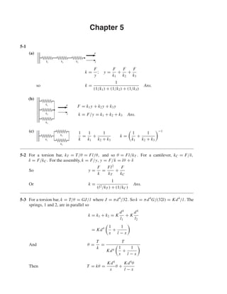
1. Chapter 5
5-1
(a)
k =
F
y
; y =
F
k1
+
F
k2
+
F
k3
so k =
1
(1/k1) + (1/k2) + (1/k3)
Ans.
(b)
F = k1y + k2y + k3y
k = F/y = k1 + k2 + k3 Ans.
(c) 1
k
=
1
k1
+
1
k2 + k3
k =
1
k1
+
1
k2 + k3
−1
5-2 For a torsion bar, kT = T/θ = Fl/θ, and so θ = Fl/kT . For a cantilever, kC = F/δ,
δ = F/kC. For the assembly, k = F/y, y = F/k = lθ + δ
So y =
F
k
=
Fl2
kT
+
F
kC
Or k =
1
(l2/kT ) + (1/kC)
Ans.
5-3 For a torsion bar, k = T/θ = GJ/l where J = πd4
/32. So k = πd4
G/(32l) = Kd4
/l . The
springs, 1 and 2, are in parallel so
k = k1 + k2 = K
d4
l1
+ K
d4
l2
= Kd4 1
x
+
1
l − x
And θ =
T
k
=
T
Kd4
1
x
+
1
l − x
Then T = kθ =
Kd4
x
θ +
Kd4
θ
l − x
k2
k1
k3
F
k2
k1
k3
y
F
k1 k2 k3 y
shi20396_ch05.qxd 8/18/03 10:59 AM Page 106

2. Chapter 5 107
Thus T1 =
Kd4
x
θ; T2 =
Kd4
θ
l − x
If x = l/2, then T1 = T2. If x < l/2, then T1 > T2
Using τ = 16T/πd3
and θ = 32Tl/(Gπd4
) gives
T =
πd3
τ
16
and so
θall =
32l
Gπd4
·
πd3
τ
16
=
2lτall
Gd
Thus, if x < l/2, the allowable twist is
θall =
2xτall
Gd
Ans.
Since k = Kd4 1
x
+
1
l − x
=
πGd4
32
1
x
+
1
l − x
Ans.
Then the maximum torque is found to be
Tmax =
πd3
xτall
16
1
x
+
1
l − x
Ans.
5-4 Both legs have the same twist angle. From Prob. 5-3, for equal shear, d is linear in x. Thus,
d1 = 0.2d2 Ans.
k =
πG
32
(0.2d2)4
0.2l
+
d4
2
0.8l
=
πG
32l
1.258d4
2 Ans.
θall =
2(0.8l)τall
Gd2
Ans.
Tmax = kθall = 0.198d3
2 τall Ans.
5-5
A = πr2
= π(r1 + x tan α)2
dδ =
Fdx
AE
=
Fdx
Eπ(r1 + x tan α)2
δ =
F
π E
l
0
dx
(r1 + x tan α)2
=
F
π E
−
1
tan α(r1 + x tan α)
l
0
=
F
π E
1
r1(r1 + l tan α)
l
x
␣
dx
F
F
r1
shi20396_ch05.qxd 8/18/03 10:59 AM Page 107

3. 108 Solutions Manual • Instructor’s Solution Manual to Accompany Mechanical Engineering Design
Then
k =
F
δ
=
π Er1(r1 + l tan α)
l
=
E A1
l
1 +
2l
d1
tan α Ans.
5-6
F = (T + dT) + w dx − T = 0
dT
dx
= −w
Solution is T = −wx + c
T|x=0 = P + wl = c
T = −wx + P + wl
T = P + w(l − x)
The infinitesmal stretch of the free body of original length dx is
dδ =
Tdx
AE
=
P + w(l − x)
AE
dx
Integrating,
δ =
l
0
[P + w(l − x)] dx
AE
δ =
Pl
AE
+
wl2
2AE
Ans.
5-7
M = wlx −
wl2
2
−
wx2
2
E I
dy
dx
=
wlx2
2
−
wl2
2
x −
wx3
6
+ C1,
dy
dx
= 0 at x = 0, ІC1 = 0
E I y =
wlx3
6
−
wl2
x2
4
−
wx4
24
+ C2, y = 0 at x = 0, ІC2 = 0
y =
wx2
24E I
(4lx − 6l2
− x2
) Ans.
l
x
dx
P
Enlarged free
body of length dx
w is cable’s weight
per foot
T ϩ dT
wdx
T
shi20396_ch05.qxd 8/18/03 10:59 AM Page 108

4. Chapter 5 109
5-8
M = M1 = MB
E I
dy
dx
= MB x + C1,
dy
dx
= 0 at x = 0, ІC1 = 0
E I y =
MB x2
2
+ C2, y = 0 at x = 0, ІC2 = 0
y =
MB x2
2E I
Ans.
5-9
ds = dx2 + dy2 = dx 1 +
dy
dx
2
Expand right-hand term by Binomial theorem
1 +
dy
dx
2 1/2
= 1 +
1
2
dy
dx
2
+ · · ·
Since dy/dx is small compared to 1, use only the first two terms,
dλ = ds − dx
= dx 1 +
1
2
dy
dx
2
− dx
=
1
2
dy
dx
2
dx
І λ =
1
2
l
0
dy
dx
2
dx Ans.
This contraction becomes important in a nonlinear, non-breaking extension spring.
5-10
y = −
4ax
l2
(l − x) = −
4ax
l
−
4a
l2
x2
dy
dx
= −
4a
l
−
8ax
l2
dy
dx
2
=
16a2
l2
−
64a2
x
l3
+
64a2
x2
l4
λ =
1
2
l
0
dy
dx
2
dx =
8
3
a2
l
Ans.
y
ds
dy
dx
␭
shi20396_ch05.qxd 8/18/03 10:59 AM Page 109

5. 110 Solutions Manual • Instructor’s Solution Manual to Accompany Mechanical Engineering Design
5-11
y = a sin
πx
l
dy
dx
=
aπ
l
cos
πx
l
dy
dx
2
=
a2
π2
l2
cos2 πx
l
λ =
1
2
l
0
dy
dx
2
dx
λ =
π2
4
a2
l
= 2.467
a2
l
Ans.
Compare result with that of Prob. 5-10. See Charles R. Mischke, Elements of Mechanical
Analysis,Addison-Wesley, Reading, Mass., 1963, pp. 244–249, for application to a nonlinear
extension spring.
5-12
I = 2(5.56) = 11.12 in4
ymax = y1 + y2 = −
wl4
8E I
+
Fa2
6E I
(a − 3l)
Here w = 50/12 = 4.167 lbf/in, and a = 7(12) = 84 in, and l = 10(12) = 120 in.
y1 = −
4.167(120)4
8(30)(106)(11.12)
= −0.324 in
y2 = −
600(84)2
[3(120) − 84]
6(30)(106)(11.12)
= −0.584 in
So ymax = −0.324 − 0.584 = −0.908 in Ans.
M0 = −Fa − (wl2
/2)
= −600(84) − [4.167(120)2
/2]
= −80 400 lbf · in
c = 4 − 1.18 = 2.82 in
σmax =
−My
I
= −
(−80 400)(−2.82)
11.12
(10−3
)
= −20.4 kpsi Ans.
σmax is at the bottom of the section.
shi20396_ch05.qxd 8/18/03 10:59 AM Page 110

6. Chapter 5 111
5-13
RO =
7
10
(800) +
5
10
(600) = 860 lbf
RC =
3
10
(800) +
5
10
(600) = 540 lbf
M1 = 860(3)(12) = 30.96(103
) lbf · in
M2 = 30.96(103
) + 60(2)(12)
= 32.40(103
) lbf · in
σmax =
Mmax
Z
⇒ 6 =
32.40
Z
Z = 5.4 in3
y|x=5ft =
F1a[l − (l/2)]
6E Il
l
2
2
+ a2
− 2l
l
2
−
F2l3
48E I
−
1
16
=
800(36)(60)
6(30)(106)I (120)
[602
+ 362
− 1202
] −
600(1203
)
48(30)(106)I
I = 23.69 in4
⇒ I/2 = 11.84 in4
Select two 6 in-8.2 lbf/ft channels; from TableA-7, I = 2(13.1) = 26.2 in4
, Z = 2(4.38) in3
ymax =
23.69
26.2
−
1
16
= −0.0565 in
σmax =
32.40
2(4.38)
= 3.70 kpsi
5-14
I =
π
64
(1.54
) = 0.2485 in4
Superpose beams A-9-6 and A-9-7,
yA =
300(24)(16)
6(30)(106)(0.2485)(40)
(162
+ 242
− 402
)
+
12(16)
24(30)(106)(0.2485)
[2(40)(162
) − 163
− 403
]
yA = −0.1006 in Ans.
y|x=20 =
300(16)(20)
6(30)(106)(0.2485)(40)
[202
+ 162
− 2(40)(20)]
−
5(12)(404)
384(30)(106)(0.2485)
= −0.1043 in Ans.
% difference =
0.1043 − 0.1006
0.1006
(100) = 3.79% Ans.
RC
M1 M2
RO
A
O
B
C
V (lbf)
M
(lbf•in)
800 lbf 600 lbf
3 ft
860
60
O
Ϫ540
2 ft 5 ft
shi20396_ch05.qxd 8/18/03 10:59 AM Page 111

7. 112 Solutions Manual • Instructor’s Solution Manual to Accompany Mechanical Engineering Design
5-15
I =
1
12
3
8
(1.53
) = 0.105 47 in4
From Table A-9-10
yC = −
Fa2
3E I
(l + a)
dyAB
dx
=
Fa
6E Il
(l2
− 3x2
)
Thus,
θA =
Fal2
6E Il
=
Fal
6E I
yD = −θAa = −
Fa2
l
6E I
With both loads,
yD = −
Fa2
l
6E I
−
Fa2
3E I
(l + a)
= −
Fa2
6E I
(3l + 2a) = −
120(102
)
6(30)(106)(0.105 47)
[3(20) + 2(10)]
= −0.050 57 in Ans.
yE =
2Fa(l/2)
6E Il
l2
−
l
2
2
=
3
24
Fal2
E I
=
3
24
120(10)(202
)
(30)(106)(0.105 47)
= 0.018 96 in Ans.
5-16 a = 36 in, l = 72 in, I = 13 in4
, E = 30 Mpsi
y =
F1a2
6E I
(a − 3l) −
F2l3
3E I
=
400(36)2
(36 − 216)
6(30)(106)(13)
−
400(72)3
3(30)(106)(13)
= −0.1675 in Ans.
5-17 I = 2(1.85) = 3.7 in4
Adding the weight of the channels, 2(5)/12 = 0.833 lbf/in,
yA = −
wl4
8E I
−
Fl3
3E I
= −
10.833(484)
8(30)(106)(3.7)
−
220(483)
3(30)(106)(3.7)
= −0.1378 in Ans.
␪A
a
D C
F
B a
EA
shi20396_ch05.qxd 8/18/03 10:59 AM Page 112

8. Chapter 5 113
5-18
I = πd4/64 = π(2)4/64 = 0.7854 in4
Tables A-9-5 and A-9-9
y = −
F2l3
48E I
+
F1a
24E I
(4a2
− 3l2
)
= −
120(40)3
48(30)(106)(0.7854)
+
80(10)(400 − 4800)
24(30)(106)(0.7854)
= −0.0130 in Ans.
5-19
(a) Useful relations
k =
F
y
=
48E I
l3
I =
kl3
48E
=
2400(48)3
48(30)106
= 0.1843 in4
From I = bh3
/12
h = 3
12(0.1843)
b
Form a table. First, Table A-17 gives likely available fractional sizes for b:
81
2, 9, 91
2, 10 in
For h:
1
2
,
9
16
,
5
8
,
11
16
,
3
4
For available b what is necessary h for required I?
(b)
I = 9(0.625)3/12 = 0.1831 in4
k =
48E I
l3
=
48(30)(106
)(0.1831)
483
= 2384 lbf/in
F =
4σ I
cl
=
4(90 000)(0.1831)
(0.625/2)(48)
= 4394 lbf
y =
F
k
=
4394
2384
= 1.84 in Ans.
choose 9"×
5
8
"
Ans.
b
3
12(0.1843)
b
8.5 0.638
9.0 0.626 ←
9.5 0.615
10.0 0.605
shi20396_ch05.qxd 8/18/03 10:59 AM Page 113

9. 114 Solutions Manual • Instructor’s Solution Manual to Accompany Mechanical Engineering Design
5-20
Torque = (600 − 80)(9/2) = 2340 lbf · in
(T2 − T1)
12
2
= T2(1 − 0.125)(6) = 2340
T2 =
2340
6(0.875)
= 446 lbf, T1 = 0.125(446) = 56 lbf
M0 = 12(680) − 33(502) + 48R2 = 0
R2 =
33(502) − 12(680)
48
= 175 lbf
R1 = 680 − 502 + 175 = 353 lbf
We will treat this as two separate problems and then sum the results.
First, consider the 680 lbf load as acting alone.
zO A = −
Fbx
6E Il
(x2
+ b2
− l2
); here b = 36",
x = 12", l = 48", F = 680 lbf
Also,
I =
πd4
64
=
π(1.5)4
64
= 0.2485 in4
zA = −
680(36)(12)(144 + 1296 − 2304)
6(30)(106)(0.2485)(48)
= +0.1182 in
zAC = −
Fa(l − x)
6E Il
(x2
+ a2
− 2lx)
where a = 12" and x = 21 + 12 = 33"
zB = −
680(12)(15)(1089 + 144 − 3168)
6(30)(106)(0.2485)(48)
= +0.1103 in
Next, consider the 502 lbf load as acting alone.
680 lbf
A CBO
R1 ϭ 510 lbf R2 ϭ 170 lbf
12" 21" 15"
z
x
R2 ϭ 175 lbf680 lbf
A C
BO
R1 ϭ 353 lbf 502 lbf
12" 21" 15"
z
x
shi20396_ch05.qxd 8/18/03 10:59 AM Page 114

10. Chapter 5 115
zO B =
Fbx
6E Il
(x2
+ b2
− l2
), where b = 15",
x = 12", l = 48", I = 0.2485 in4
Then, zA =
502(15)(12)(144 + 225 − 2304)
6(30)(106)(0.2485)(48)
= −0.081 44 in
For zB use x = 33"
zB =
502(15)(33)(1089 + 225 − 2304)
6(30)(106)(0.2485)(48)
= −0.1146 in
Therefore, by superposition
zA = +0.1182 − 0.0814 = +0.0368 in Ans.
zB = +0.1103 − 0.1146 = −0.0043 in Ans.
5-21
(a) Calculate torques and moment of inertia
T = (400 − 50)(16/2) = 2800 lbf · in
(8T2 − T2)(10/2) = 2800 ⇒ T2 = 80 lbf, T1 = 8(80) = 640 lbf
I =
π
64
(1.254
) = 0.1198 in4
Due to 720 lbf, flip beamA-9-6 such that yAB → b = 9, x = 0,l = 20, F = −720 lbf
θB =
dy
dx x=0
= −
Fb
6E Il
(3x2
+ b2
− l2
)
= −
−720(9)
6(30)(106)(0.1198)(20)
(0 + 81 − 400) = −4.793(10−3
) rad
yC = −12θB = −0.057 52 in
Due to 450 lbf, use beam A-9-10,
yC = −
Fa2
3E I
(l + a) = −
450(144)(32)
3(30)(106)(0.1198)
= −0.1923 in
450 lbf720 lbf
9" 11" 12"
O
y
A
B
C
RO
RB
A CB
O
R1 R2
12"
502 lbf
21" 15"
z
x
shi20396_ch05.qxd 8/18/03 10:59 AM Page 115

11. 116 Solutions Manual • Instructor’s Solution Manual to Accompany Mechanical Engineering Design
Adding the two deflections,
yC = −0.057 52 − 0.1923 = −0.2498 in Ans.
(b) At O:
Due to 450 lbf:
dy
dx x=0
=
Fa
6E Il
(l2
− 3x2
)
x=0
=
Fal
6E I
θO = −
720(11)(0 + 112
− 400)
6(30)(106)(0.1198)(20)
+
450(12)(20)
6(30)(106)(0.1198)
= 0.010 13 rad = 0.5805◦
At B:
θB = −4.793(10−3
) +
450(12)
6(30)(106)(0.1198)(20)
[202
− 3(202
)]
= −0.014 81 rad = 0.8485◦
I = 0.1198
0.8485◦
0.06◦
= 1.694 in4
d =
64I
π
1/4
=
64(1.694)
π
1/4
= 2.424 in
Use d = 2.5 in Ans.
I =
π
64
(2.54
) = 1.917 in4
yC = −0.2498
0.1198
1.917
= −0.015 61 in Ans.
5-22
(a) l = 36(12) = 432 in
ymax = −
5wl4
384E I
= −
5(5000/12)(432)4
384(30)(106)(5450)
= −1.16 in
The frame is bowed up 1.16 in with respect to the bolsters. It is fabricated upside down
and then inverted. Ans.
(b) The equation in xy-coordinates is for the center sill neutral surface
y =
wx
24E I
(2lx2
− x3
− l3
) Ans.
y
x
l
shi20396_ch05.qxd 8/18/03 10:59 AM Page 116

12. Chapter 5 117
Differentiating this equation and solving for the slope at the left bolster gives
Thus,
dy
dx
=
w
24E I
(6lx2
− 4x3
− l3
)
dy
dx x=0
= −
wl3
24E I
= −
(5000/12)(432)3
24(30)(106)(5450)
= −0.008 57
The slope at the right bolster is 0.00857, so equation at left end is y = −0.008 57x and
at the right end is y = 0.008 57(x − l). Ans.
5-23 From Table A-9-6,
yL =
Fbx
6E Il
(x2
+ b2
− l2
)
yL =
Fb
6E Il
(x3
+ b2
x − l2
x)
dyL
dx
=
Fb
6E Il
(3x2
+ b2
− l2
)
dyL
dx x=0
=
Fb(b2
− l2
)
6E Il
Let ξ =
Fb(b2 − l2)
6E Il
And set I =
πd4
L
64
And solve for dL
dL =
32Fb(b2 − l2)
3π Elξ
1/4
Ans.
For the other end view, observe the figure of Table A-9-6 from the back of the page, noting
that a and b interchange as do x and −x
dR =
32Fa(l2 − a2)
3π Elξ
1/4
Ans.
For a uniform diameter shaft the necessary diameter is the larger of dL and dR.
shi20396_ch05.qxd 8/18/03 10:59 AM Page 117

13. 118 Solutions Manual • Instructor’s Solution Manual to Accompany Mechanical Engineering Design
5-24 Incorporating a design factor into the solution for dL of Prob. 5-23,
d =
32n
3π Elξ
Fb(l2
− b2
)
1/4
= (mm 10−3
)
kN mm3
GPa mm
103
(10−9
)
109(10−3)
1/4
d = 4
32(1.28)(3.5)(150)|(2502 − 1502)|
3π(207)(250)(0.001)
10−12
= 36.4 mm Ans.
5-25 The maximum occurs in the right section. Flip beam A-9-6 and use
y =
Fbx
6E Il
(x2
+ b2
− l2
) where b = 100 mm
dy
dx
=
Fb
6E Il
(3x2
+ b2
− l2
) = 0
Solving for x,
x =
l2 − b2
3
=
2502 − 1002
3
= 132.29 mm from right
y =
3.5(103
)(0.1)(0.132 29)
6(207)(109)(π/64)(0.03644)(0.25)
[0.132 292
+ 0.12
− 0.252
](103
)
= −0.0606 mm Ans.
5-26
x
y
z
F1
a2
b2
b1
a1
F2
3.5 kN
100
250
150
d
The slope at x = 0 due to F1 in the xy plane is
θxy =
F1b1 b2
1 − l2
6E Il
and in the xz plane due to F2 is
θxz =
F2b2 b2
2 − l2
6E Il
For small angles, the slopes add as vectors. Thus
θL = θ2
xy + θ2
xz
1/2
=


F1b1 b2
1 − l2
6E Il
2
+
F2b2 b2
2 − l2
6E Il
2


1/2
shi20396_ch05.qxd 8/18/03 10:59 AM Page 118

14. Chapter 5 119
Designating the slope constraint as ξ, we then have
ξ = |θL| =
1
6E Il
Fi bi b2
i − l2 2 1/2
Setting I = πd4
/64 and solving for d
d =
32
3π Elξ
Fi bi b2
i − l2 2 1/2 1/4
For the LH bearing, E = 30 Mpsi, ξ = 0.001, b1 = 12, b2 = 6, and l = 16. The result is
dL =1.31 in. Using a similar flip beam procedure, we get dR = 1.36 in for the RH bearing.
So use d = 1 3/8 in Ans.
5-27 For the xy plane, use yBC of Table A-9-6
y =
100(4)(16 − 8)
6(30)(106)(16)
[82
+ 42
− 2(16)8] = −1.956(10−4
) in
For the xz plane use yAB
z =
300(6)(8)
6(30)(106)(16)
[82
+ 62
− 162
] = −7.8(10−4
) in
δ = (−1.956j − 7.8k)(10−4
) in
|δ| = 8.04(10−4
) in Ans.
5-28
dL =
32n
3π Elξ
Fi bi b2
i − l2 2 1/2 1/4
=
32(1.5)
3π(29.8)(106)(10)(0.001)
[800(6)(62
− 102
)]2
+ [600(3)(32
− 102
)]2 1/2
1/4
= 1.56 in
dR =
32(1.5)
3π(29.8)(106)(10)(0.001)
[800(4)(102
− 42
)]2
+ [600(7)(102
− 72
)]2 1/2
1/4
= 1.56 in choose d ≥ 1.56 in Ans.
5-29 From Table A-9-8 we have
yL =
MB x
6E Il
(x2
+ 3a2
− 6al + 2l2
)
dyL
dx
=
MB
6E Il
(3x2
+ 3a2
− 6al + 2l2
)
shi20396_ch05.qxd 8/18/03 10:59 AM Page 119

15. 120 Solutions Manual • Instructor’s Solution Manual to Accompany Mechanical Engineering Design
At x = 0, the LH slope is
θL =
dyL
dx
=
MB
6E Il
(3a2
− 6al + 2l2
)
from which
ξ = |θL| =
MB
6E Il
(l2
− 3b2
)
Setting I = πd4
/64 and solving for d
d =
32MB(l2
− 3b2
)
3π Elξ
1/4
For a multiplicity of moments, the slopes add vectorially and
dL =
32
3π Elξ
Mi l2
− 3b2
i
2 1/2 1/4
dR =
32
3π Elξ
Mi 3a2
i − l2 2 1/2 1/4
The greatest slope is at the LH bearing. So
d =
32(1200)[92
− 3(42
)]
3π(30)(106)(9)(0.002)
1/4
= 0.706 in
So use d = 3/4 in Ans.
5-30
6FAC = 18(80)
FAC = 240 lbf
RO = 160 lbf
I =
1
12
(0.25)(23
) = 0.1667 in4
Initially, ignore the stretch of AC. From Table A-9-10
yB1 = −
Fa2
3E I
(l + a) = −
80(122
)
3(10)(106)(0.1667)
(6 + 12) = −0.041 47 in
Stretch of AC: δ =
FL
AE AC
=
240(12)
(π/4)(1/2)2
(10)(106)
= 1.4668(10−3
) in
Due to stretch of AC
By superposition,
yB2 = −3δ = −4.400(10−3
) in
yB = −0.041 47 − 0.0044 = −0.045 87 in Ans.
80 lbfFAC
126
B
RO
shi20396_ch05.qxd 8/18/03 10:59 AM Page 120

16. Chapter 5 121
5-31
θ =
T L
JG
=
(0.1F)(1.5)
(π/32)(0.0124)(79.3)(109)
= 9.292(10−4
)F
Due to twist
δB1 = 0.1(θ) = 9.292(10−5
)F
Due to bending
δB2 =
FL3
3E I
=
F(0.13
)
3(207)(109)(π/64)(0.0124)
= 1.582(10−6
)F
δB = 1.582(10−6
)F + 9.292(10−5
)F = 9.450(10−5
)F
k =
1
9.450(10−5)
= 10.58(103
) N/m = 10.58 kN/m Ans.
5-32
R1 =
Fb
l
R2 =
Fa
l
δ1 =
R1
k1
δ2 =
R2
k2
Spring deflection
yS = −δ1 +
δ1 − δ2
l
x = −
Fb
k1l
+
Fb
k1l2
−
Fa
k2l2
x
yAB =
Fbx
6E Il
(x2
+ b2
− l2
) +
Fx
l2
b
k1
−
a
k2
−
Fb
k1l
Ans.
yBC =
Fa(l − x)
6E Il
(x2
+ a2
− 2lx) +
Fx
l2
b
k1
−
a
k2
−
Fb
k1l
Ans.
5-33 See Prob. 5-32 for deflection due to springs. Replace Fb/l and Fa/l with wl/2
yS = −
wl
2k1
+
wl
2k1l
−
wl
2k2l
x =
wx
2
1
k1
+
1
k2
−
wl
2k1
y =
wx
24E I
(2lx2
− x3
− l3
) +
wx
2
1
k1
+
1
k2
−
wl
2k1
Ans.
F
ba CA B
l
R2
␦2␦1
R1
shi20396_ch05.qxd 8/18/03 10:59 AM Page 121

17. 122 Solutions Manual • Instructor’s Solution Manual to Accompany Mechanical Engineering Design
5-34 Let the load be at x > l/2. The maximum deflection will be in Section AB (Table A-9-10)
yAB =
Fbx
6E Il
(x2
+ b2
− l2
)
dyAB
dx
=
Fb
6E Il
(3x2
+ b2
− l2
) = 0 ⇒ 3x2
+ b2
− l2
= 0
x =
l2 − b2
3
, xmax =
l2
3
= 0.577l Ans.
For x < l/2 xmin = l − 0.577l = 0.423l Ans.
5-35
MO = 50(10)(60) + 600(84)
= 80 400 lbf · in
RO = 50(10) + 600 = 1100 lbf
I = 11.12 in4
from Prob. 5-12
M = −80 400 + 1100x −
4.167x2
2
− 600 x − 84 1
E I
dy
dx
= −80 400x + 550x2
− 0.6944x3
− 300 x − 84 2
+ C1
dy
dx
= 0 at x = 0 І C1 = 0
E I y = −402 00x2
+ 183.33x3
− 0.1736x4
− 100 x − 84 3
+ C2
y = 0 at x = 0 І C2 = 0
yB =
1
30(106)(11.12)
[−40 200(1202
) + 183.33(1203
)
− 0.1736(1204
) − 100(120 − 84)3
]
= −0.9075 in Ans.
5-36 See Prob. 5-13 for reactions: RO = 860 lbf, RC = 540 lbf
M = 860x − 800 x − 36 1
− 600 x − 60 1
E I
dy
dx
= 430x2
− 400 x − 36 2
− 300 x − 60 2
+ C1
E I y = 143.33x3
− 133.33 x − 36 3
− 100 x − 60 3
+ C1x + C2
y = 0 at x = 0 ⇒ C2 = 0
y = 0 at x = 120 in ⇒ C1 = −1.2254(106
) lbf · in2
Substituting C1 and C2 and evaluating at x = 60,
E I y = 30(106
)I −
1
16
= 143.33(603
) − 133.33(60 − 36)3
− 1.2254(106
)(60)
I = 23.68 in4
Agrees with Prob. 5-13. The rest of the solution is the same.
10'
7'
RO
600 lbf50 lbf/ft
MO
O
A
B
shi20396_ch05.qxd 8/18/03 10:59 AM Page 122

18. Chapter 5 123
5-37
I = 0.2485 in4
RO = 12(20) +
24
40
(300) = 420 lbf
M = 420x −
12
2
x2
− 300 x − 16 1
E I
dy
dx
= 210x2
− 2x3
− 150 x − 16 2
+ C1
E I y = 70x3
− 0.5x4
− 50 x − 16 3
+ C1x + C2
y = 0 at x = 0 ⇒ C2 = 0
y = 0 at x = 40 in ⇒ C1 = −6.272(104
) lbf · in2
Substituting for C1 and C2 and evaluating at x = 16,
yA =
1
30(106)(0.2485)
[70(163
) − 0.5(164
) − 6.272(104
)(16)]
= −0.1006 in Ans.
y|x=20 =
1
30(106)(0.2485)
[70(203
) − 0.5(204
) − 50(20 − 16)3
− 6.272(104
)(20)]
= 0.1043 in Ans.
3.7% difference Ans.
5-38
R1 =
w[(l + a)/2][(l − a)/2)]
l
=
w
4l
(l2
− a2
)
R2 =
w
2
(l + a) −
w
4l
(l2
− a2
) =
w
4l
(l + a)2
M =
w
4l
(l2
− a2
)x −
wx2
2
+
w
4l
(l + a)2
x − l 1
E I
dy
dx
=
w
8l
(l2
− a2
)x2
−
w
6
x3
+
w
8l
(l + a)2
x − l 2
+ C1
E I y =
w
24l
(l2
− a2
)x3
−
w
24
x4
+
w
24l
(l + a)2
x − l 3
+ C1x + C2
y = 0 at x = 0 ⇒ C2 = 0
y = 0 at x = l
0 =
w
24l
(l2
− a2
)l3
−
w
24
l4
+ C1l ⇒ C1 =
wa2
l
24
y =
w
24E Il
[(l2
− a2
)x3
− lx4
+ (l + a)2
x − l 3
+ a2
l2
x] Ans.
a
w
l ϩ a
2΂ ΃
l Ϫ a
2
shi20396_ch05.qxd 8/18/03 10:59 AM Page 123

19. 124 Solutions Manual • Instructor’s Solution Manual to Accompany Mechanical Engineering Design
5-39 From Prob. 5-15, RA = RB = 120 lbf, and I = 0.105 47 in4
First half of beam,
M = −120x + 120 x − 10 1
E I
dy
dx
= −60x2
+ 60 x − 10 2
+ C1
dy/dx = 0 at x = 20 in ⇒ 0 = −60(202
) + 60(20 −10)2
+ C1 ⇒ C1 = 1.8(104
) lbf · in2
E I y = −20x3
+ 20 x − 10 3
+ 1.8(104
)x + C2
y = 0 at x = 10 in ⇒ C2 = −1.6(105
) lbf · in3
y|x=0 =
1
30(106)(0.105 47)
(−1.6)(105
)
= −0.050 57 in Ans.
y|x=20 =
1
30(106)(0.105 47)
[−20(203
) + 20(20 − 10)3
+ 1.8(104
)(20) − 1.6(105
)]
= 0.018 96 in Ans.
5-40 From Prob. 5-30, RO = 160 lbf ↓, FAC = 240 lbf I = 0.1667 in4
M = −160x + 240 x − 6 1
E I
dy
dx
= −80x2
+ 120 x − 6 2
+ C1
E I y = −26.67x3
+ 40 x − 6 3
+ C1x + C2
y = 0 at x = 0 ⇒ C2 = 0
yA = −
FL
AE AC
= −
240(12)
(π/4)(1/2)2(10)(106)
= −1.4668(10−3
) in
at x = 6
10(106
)(0.1667)(−1.4668)(10−3
) = −26.67(63
) + C1(6)
C1 = 552.58 lbf · in2
yB =
1
10(106)(0.1667)
[−26.67(183
) + 40(18 − 6)3
+ 552.58(18)]
= −0.045 87 in Ans.
5-41
I1 =
π
64
(1.54
) = 0.2485 in4
I2 =
π
64
(24
) = 0.7854 in4
R1 =
200
2
(12) = 1200 lbf
For 0 ≤ x ≤ 16 in, M = 1200x −
200
2
x − 4 2 x
MրI
shi20396_ch05.qxd 8/18/03 10:59 AM Page 124

20. Chapter 5 125
M
I
=
1200x
I1
− 4800
1
I1
−
1
I2
x − 4 0
− 1200
1
I1
−
1
I2
x − 4 1
−
100
I2
x − 4 2
= 4829x − 13 204 x − 4 0
− 3301.1 x − 4 1
− 127.32 x − 4 2
E
dy
dx
= 2414.5x2
− 13 204 x − 4 1
− 1651 x − 4 2
− 42.44 x − 4 3
+ C1
Boundary Condition:
dy
dx
= 0 at x = 10 in
0 = 2414.5(102
) − 13 204(10 − 4)1
− 1651(10 − 4)2
− 42.44(10 − 4)3
+ C1
C1 = −9.362(104
)
Ey = 804.83x3
− 6602 x − 4 2
− 550.3 x − 4 3
− 10.61 x − 4 4
− 9.362(104
)x + C2
y = 0 at x = 0 ⇒ C2 = 0
For 0 ≤ x ≤ 16 in
y =
1
30(106)
[804.83x3
− 6602 x − 4 2
− 550.3 x − 4 3
− 10.61 x − 4 4
− 9.362(104
)x] Ans.
at x = 10 in
y|x=10 =
1
30(106)
[804.83(103
) − 6602(10 − 4)2
− 550.3(10 − 4)3
− 10.61(10 − 4)4
− 9.362(104
)(10)]
= −0.016 72 in Ans.
5-42 Define δi j as the deflection in the direction of the load at station i due to a unit load at station j.
If U is the potential energy of strain for a body obeying Hooke’s law, apply P1 first. Then
U =
1
2
P1(P1δ11)
When the second load is added, U becomes
U =
1
2
P1(P1δ11) +
1
2
P2(P2 δ22) + P1(P2 δ12)
For loading in the reverse order
U =
1
2
P2(P2 δ22) +
1
2
P1(P1δ11) + P2(P1 δ21)
Since the order of loading is immaterial U = U and
P1 P2δ12 = P2 P1δ21 when P1 = P2, δ12 = δ21
which states that the deflection at station 1 due to a unit load at station 2 is the same as the
deflection at station 2 due to a unit load at 1. δ is sometimes called an influence coefficient.
shi20396_ch05.qxd 8/18/03 10:59 AM Page 125

21. 126 Solutions Manual • Instructor’s Solution Manual to Accompany Mechanical Engineering Design
5-43
(a) From Table A-9-10
yAB =
Fcx(l2
− x2
)
6E Il
δ12 =
y
F x=a
=
ca(l2
− a2
)
6E Il
y2 = Fδ21 = Fδ12 =
Fca(l2
− a2
)
6E Il
Substituting I =
πd4
64
y2 =
400(7)(9)(232
− 92
)(64)
6(30)(106)(π)(2)4(23)
= 0.00347 in Ans.
(b) The slope of the shaft at left bearing at x = 0 is
θ =
Fb(b2 − l2)
6E Il
Viewing the illustration in Section 6 of Table A-9 from the back of the page provides
the correct view of this problem. Noting that a is to be interchanged with b and −x
with x leads to
θ =
Fa(l2 − a2)
6E Il
=
Fa(l2 − a2)(64)
6Eπd4l
θ =
400(9)(232
− 92
)(64)
6(30)(106)(π)(2)4(23)
= 0.000 496 in/in
So y2 = 7θ = 7(0.000 496) = 0.00347 in Ans.
5-44 Place a dummy load Q at the center. Then,
M =
wx
2
(l − x) +
Qx
2
U = 2
l/2
0
M2
dx
2E I
, ymax =
∂U
∂Q Q=0
ymax = 2
l/2
0
2M
2E I
∂M
∂Q
dx
Q=0
ymax =
2
E I
l/2
0
wx
2
(l − x) +
Qx
2
x
2
dx
Q=0
Set Q = 0 and integrate
400 lbf
9"
a
A B
c
21
x
b
7"
23"
y
shi20396_ch05.qxd 8/18/03 10:59 AM Page 126

22. Chapter 5 127
ymax =
w
2E I
lx3
3
−
x4
4
l/2
0
ymax =
5wl4
384E I
Ans.
5-45
I = 2(1.85) = 3.7 in4
Adding weight of channels of 0.833 lbf · in,
M = −Fx −
10.833
2
x2
= −Fx − 5.417x2 ∂M
∂F
= −x
δB =
1
E I
48
0
M
∂M
∂F
dx =
1
E I
48
0
(Fx + 5.417x2
)(x) dx
=
(220/3)(483
) + (5.417/4)(484
)
30(106)(3.7)
= 0.1378 in in direction of 220 lbf
ІyB = −0.1378 in Ans.
5-46
IO B =
1
12
(0.25)(23
) = 0.1667 in4
, AAC =
π
4
1
2
2
= 0.196 35 in2
FAC = 3F,
∂FAC
∂F
= 3
right left
M = −F ¯x M = −2Fx
∂M
∂F
= −¯x
∂M
∂F
= −2x
U =
1
2E I
l
0
M2
dx +
F2
AC LAC
2AAC E
δB =
∂U
∂F
=
1
E I
l
0
M
∂M
∂F
dx +
FAC(∂FAC/∂F)LAC
AAC E
=
1
E I
12
0
−F ¯x(−¯x) d ¯x +
6
0
(−2Fx)(−2x) dx +
3F(3)(12)
AAC E
=
1
E I
F
3
(123
) + 4F
63
3
+
108F
AAC E
=
864F
E I
+
108F
AAC E
=
864(80)
10(106)(0.1667)
+
108(80)
0.196 35(10)(106)
= 0.045 86 in Ans.
FAC ϭ 3F
O
A B
F2F
x
6" 12"
x¯
shi20396_ch05.qxd 8/18/03 10:59 AM Page 127

23. 128 Solutions Manual • Instructor’s Solution Manual to Accompany Mechanical Engineering Design
5-47
Torsion T = 0.1F
∂T
∂F
= 0.1
Bending M = −F ¯x
∂M
∂F
= −¯x
U =
1
2E I
M2
dx +
T2
L
2JG
δB =
∂U
∂F
=
1
E I
M
∂M
∂F
dx +
T(∂T/∂F)L
JG
=
1
E I
0.1
0
−F ¯x(−¯x) d ¯x +
0.1F(0.1)(1.5)
JG
=
F
3E I
(0.13
) +
0.015F
JG
Where
I =
π
64
(0.012)4
= 1.0179(10−9
) m4
J = 2I = 2.0358(10−9
) m4
δB = F
0.001
3(207)(109)(1.0179)(10−9)
+
0.015
2.0358(10−9)(79.3)(109)
= 9.45(10−5
)F
k =
1
9.45(10−5)
= 10.58(103
) N/m = 10.58 kN/m Ans.
5-48 From Prob. 5-41, I1 = 0.2485 in4
, I2 = 0.7854 in4
For a dummy load ↑ Q at the center
0 ≤ x ≤ 10 in M = 1200x −
Q
2
x −
200
2
x − 4 2
,
∂M
∂Q
=
−x
2
y|x=10 =
∂U
∂Q Q=0
=
2
E
1
I1
4
0
(1200x) −
x
2
dx +
1
I2
10
4
[1200x − 100(x − 4)2
] −
x
2
dx
=
2
E
−
200(43
)
I1
−
1.566(105
)
I2
= −
2
30(106)
1.28(104
)
0.2485
+
1.566(105
)
0.7854
= −0.016 73 in Ans.
x
F
shi20396_ch05.qxd 8/18/03 10:59 AM Page 128

24. Chapter 5 129
5-49
AB
M = Fx
∂M
∂F
= x
OA N =
3
5
F
∂N
∂F
=
3
5
T =
4
5
Fa
∂T
∂F
=
4
5
a
M1 =
4
5
F ¯x
∂M1
∂F
=
4
5
¯x
M2 =
3
5
Fa
∂M2
∂F
=
3
5
a
δB =
∂u
∂F
=
1
E I
a
0
Fx(x) dx +
(3/5)F(3/5)l
AE
+
(4/5)Fa(4a/5)l
JG
+
1
E I
l
0
4
5
F ¯x
4
5
¯x d ¯x +
1
E I
l
0
3
5
Fa
3
5
a d ¯x
=
Fa3
3E I
+
9
25
Fl
AE
+
16
25
Fa2
l
JG
+
16
75
Fl3
E I
+
9
25
Fa2
l
E I
I =
π
64
d4
, J = 2I, A =
π
4
d2
δB =
64Fa3
3Eπd4
+
9
25
4Fl
πd2 E
+
16
25
32Fa2
l
πd4G
+
16
75
64Fl3
Eπd4
+
9
25
64Fa2
l
Eπd4
=
4F
75π Ed4
400a3
+ 27ld2
+ 384a2
l
E
G
+ 256l3
+ 432a2
l Ans.
a
O
B
A
F
3
5
F
4
5
a
B
x
A
F
3
5
F
4
5
O
l
l
A
F
3
5
Fa
3
5
Fa
4
5
F
4
5
x
shi20396_ch05.qxd 8/18/03 10:59 AM Page 129

25. 130 Solutions Manual • Instructor’s Solution Manual to Accompany Mechanical Engineering Design
5-50 The force applied to the copper and steel wire assembly is Fc + Fs = 250 lbf
Since δc = δs
FcL
3(π/4)(0.0801)2(17.2)(106)
=
Fs L
(π/4)(0.0625)2(30)(106)
Fc = 2.825Fs
∴ 3.825Fs = 250 ⇒ Fs = 65.36 lbf, Fc = 2.825Fs = 184.64 lbf
σc =
184.64
3(π/4)(0.0801)2
= 12 200 psi = 12.2 kpsi Ans.
σs =
65.36
(π/4)(0.06252)
= 21 300 psi = 21.3 kpsi Ans.
5-51
(a) Bolt stress σb = 0.9(85) = 76.5 kpsi Ans.
Bolt force Fb = 6(76.5)
π
4
(0.3752
) = 50.69 kips
Cylinder stress σc = −
Fb
Ac
= −
50.69
(π/4)(4.52 − 42)
= −15.19 kpsi Ans.
(b) Force from pressure
P =
π D2
4
p =
π(42
)
4
(600) = 7540 lbf = 7.54 kip
Fx = 0
Pb + Pc = 7.54 (1)
Since δc = δb ,
PcL
(π/4)(4.52 − 42)E
=
PbL
6(π/4)(0.3752)E
Pc = 5.037Pb (2)
Substituting into Eq. (1)
6.037Pb = 7.54 ⇒ Pb = 1.249 kip; and from Eq (2), Pc = 6.291 kip
Using the results of (a) above, the total bolt and cylinder stresses are
σb = 76.5 +
1.249
6(π/4)(0.3752)
= 78.4 kpsi Ans.
σc = −15.19 +
6.291
(π/4)(4.52 − 42)
= −13.3 kpsi Ans.
6 bolts
50.69 Ϫ Pc
50.69 ϩ Pb
x
P ϭ 7.54 kip
shi20396_ch05.qxd 8/18/03 10:59 AM Page 130

26. Chapter 5 131
5-52
T = Tc + Ts and θc = θs
Also,
TcL
(G J)c
=
Ts L
(G J)s
Tc =
(G J)c
(G J)s
Ts
Substituting into equation for T ,
T = 1 +
(G J)c
(G J)s
Ts
%Ts =
Ts
T
=
(G J)s
(G J)s + (G J)c
Ans.
5-53
RO + RB = W (1)
δO A = δAB (2)
20RO
AE
=
30RB
AE
, RO =
3
2
RB
3
2
RB + RB = 800
RB =
1600
5
= 320 lbf Ans.
RO = 800 − 320 = 480 lbf Ans.
σO = −
480
1
= −480 psi Ans.
σB = +
320
1
= 320 psi Ans.
5-54 Since θO A = θAB
TO A(4)
G J
=
TAB(6)
G J
, TO A =
3
2
TAB
Also TO A + TAB = T
TAB
3
2
+ 1 = T, TAB =
T
2.5
Ans.
TO A =
3
2
TAB =
3T
5
Ans.
RB
W ϭ 800 lbf
30"
20"
RO
A
B
O
shi20396_ch05.qxd 8/18/03 10:59 AM Page 131

27. 132 Solutions Manual • Instructor’s Solution Manual to Accompany Mechanical Engineering Design
5-55
F1 = F2 ⇒
T1
r1
=
T2
r2
⇒
T1
1.25
=
T2
3
T2 =
3
1.25
T1
∴ θ1 +
3
1.25
θ2 =
4π
180
rad
T1(48)
(π/32)(7/8)4(11.5)(106)
+
3
1.25
(3/1.25)T1(48)
(π/32)(1.25)4(11.5)(106)
=
4π
180
T1 = 403.9 lbf · in
T2 =
3
1.25
T1 = 969.4 lbf · in
τ1 =
16T1
πd3
=
16(403.9)
π(7/8)3
= 3071 psi Ans.
τ2 =
16(969.4)
π(1.25)3
= 2528 psi Ans.
5-56
(1) Arbitrarily, choose RC as redundant reaction
(2) Fx = 0, 10(103
) − 5(103
) − RO − RC = 0
RO + RC = 5(103
) lbf
(3) δC =
[10(103
) − 5(103
) − RC]20
AE
−
[5(103
) + RC]
AE
(10) −
RC(15)
AE
= 0
−45RC + 5(104
) = 0 ⇒ RC = 1111 lbf Ans.
RO = 5000 − 1111 = 3889 lbf Ans.
5-57
(1) Choose RB as redundant reaction
(2) RB + RC = wl (a) RB(l − a) −
wl2
2
+ MC = 0 (b)
RB
A
x
w
RC
CB
MC
a
l
10 kip 5 kip
FA FB RCRO x
shi20396_ch05.qxd 8/18/03 10:59 AM Page 132

28. Chapter 5 133
(3) yB =
RB(l − a)3
3E I
+
w(l − a)2
24E I
[4l(l − a) − (l − a)2
− 6l2
] = 0
RB =
w
8(l − a)
[6l2
− 4l(l − a) + (l − a)2
]
=
w
8(l − a)
(3l2
+ 2al + a2
) Ans.
Substituting,
Eq. (a) RC = wl − RB =
w
8(l − a)
(5l2
− 10al − a2
) Ans.
Eq. (b) MC =
wl2
2
− RB(l − a) =
w
8
(l2
− 2al − a2
) Ans.
5-58
M = −
wx2
2
+ RB x − a 1
,
∂M
∂ RB
= x − a 1
∂U
∂ RB
=
1
E I
l
0
M
∂M
∂ RB
dx
=
1
E I
a
0
−wx2
2
(0) dx +
1
E I
l
a
−wx2
2
+ RB(x − a) (x − a) dx = 0
−
w
2
1
4
(l4
− a4
) −
a
3
(l3
− a3
) +
RB
3
(l − a)3
− (a − a)3
= 0
RB =
w
(l − a)3
[3(L4
− a4
) − 4a(l3
− a3
)] =
w
8(l − a)
(3l2
+ 2al + a2
) Ans.
RC = wl − RB =
w
8(l − a)
(5l2
− 10al − a2
) Ans.
MC =
wl2
2
− RB(l − a) =
w
8
(l2
− 2al − a2
) Ans.
5-59
A =
π
4
(0.0122
) = 1.131(10−4
) m2
(1) RA + FBE + FDF = 20 kN (a)
MA = 3FDF − 2(20) + FBE = 0
FBE + 3FDF = 40 kN (b)
FBE FDF
D
C
20 kN
500500 500
B
A
RA
RB
A
a B C
RC
MC
x
w
shi20396_ch05.qxd 8/18/03 10:59 AM Page 133

29. 134 Solutions Manual • Instructor’s Solution Manual to Accompany Mechanical Engineering Design
(2) M = RAx + FBE x − 0.5 1
− 20(103
) x − 1 1
E I
dy
dx
= RA
x2
2
+
FBE
2
x − 0.5 2
− 10(103
) x − 1 2
+ C1
E I y = RA
x3
6
+
FBE
6
x − 0.5 3
−
10
3
(103
) x − 1 3
+ C1x + C2
(3) y = 0 at x = 0 І C2 = 0
yB = −
Fl
AE BE
= −
FBE(1)
1.131(10−4)209(109)
= −4.2305(10−8
)FBE
Substituting and evaluating at x = 0.5 m
E I yB = 209(109
)(8)(10−7
)(−4.2305)(10−8
)FBE = RA
0.53
6
+ C1(0.5)
2.0833(10−2
)RA + 7.0734(10−3
)FBE + 0.5C1 = 0 (c)
yD = −
Fl
AE DF
= −
FDF(1)
1.131(10−4)(209)(109)
= −4.2305(10−8
)FDF
Substituting and evaluating at x = 1.5 m
E I yD =−7.0734(10−3
)FDF = RA
1.53
6
+
FBE
6
(1.5 − 0.5)3
−
10
3
(103
)(1.5 − 1)3
+1.5C1
0.5625RA + 0.166 67FBE + 7.0734(10−3
)FDF + 1.5C1 = 416.67 (d)




1 1 1 0
0 1 3 0
2.0833(10−2
) 7.0734(10−3
) 0 0.5
0.5625 0.166 67 7.0734(10−3
) 1.5







RA
FBE
FDF
C1



=



20 000
40 000
0
416.67



Solve simultaneously or use software
RA = −3885 N, FBE = 15 830 N, FDF = 8058 N, C1 = −62.045 N · m2
σBE =
15 830
(π/4)(122)
= 140 MPa Ans., σDF =
8058
(π/4)(122)
= 71.2 MPa Ans.
E I = 209(109
)(8)(10−7
) = 167.2(103
) N · m2
y =
1
167.2(103)
−
3885
6
x3
+
15 830
6
x − 0.5 3
−
10
3
(103
) x − 1 3
− 62.045x
B: x = 0.5 m, yB = −6.70(10−4
) m = −0.670 mm Ans.
C: x = 1 m, yC =
1
167.2(103)
−
3885
6
(13
) +
15 830
6
(1 − 0.5)3
− 62.045(1)
= −2.27(10−3
) m = −2.27 mm Ans.
D: x = 1.5, yD =
1
167.2(103)
−
3885
6
(1.53
) +
15 830
6
(1.5 − 0.5)3
−
10
3
(103
)(1.5 − 1)3
− 62.045(1.5)
= −3.39(10−4
) m = −0.339 mm Ans.
shi20396_ch05.qxd 8/18/03 10:59 AM Page 134

30. Chapter 5 135
5-60
E I = 30(106
)(0.050) = 1.5(106
) lbf · in2
(1) RC + FBE − FFD = 500 (a)
3RC + 6FBE = 9(500) = 4500 (b)
(2) M = −500x + FBE x − 3 1
+ RC x − 6 1
E I
dy
dx
= −250x2
+
FBE
2
x − 3 2
+
RC
2
x − 6 2
+ C1
E I y = −
250
3
x3
+
FBE
6
x − 3 3
+
RC
6
x − 6 3
+ C1x + C2
yB =
Fl
AE BE
= −
FBE(2)
(π/4)(5/16)2(30)(106)
= −8.692(10−7
)FBE
Substituting and evaluating at x = 3 in
E I yB = 1.5(106
)[−8.692(10−7
)FBE] = −
250
3
(33
) + 3C1 + C2
1.3038FBE + 3C1 + C2 = 2250 (c)
Since y = 0 at x = 6 in
E I y|=0 = −
250
3
(63
) +
FBE
6
(6 − 3)3
+ 6C1 + C2
4.5FBE + 6C1 + C2 = 1.8(104
) (d)
yD =
Fl
AE DF
=
FDF(2.5)
(π/4)(5/16)2(30)(106)
= 1.0865(10−6
)FDF
Substituting and evaluating at x = 9 in
E I yD = 1.5(106
)[1.0865(10−6
)FDF] = −
250
3
(93
) +
FBE
6
(9 − 3)3
+
RC
6
(9 − 6)3
+ 9C1 + C2
4.5RC + 36FBE − 1.6297FDF + 9C1 + C2 = 6.075(104
) (e)






1 1 −1 0 0
3 6 0 0 0
0 1.3038 0 3 1
0 4.5 0 6 1
4.5 36 −1.6297 9 1









RC
FBE
FDF
C1
C2



=



500
4500
2250
1.8(104
)
6.075(104
)



RC = −590.4 lbf, FBE = 1045.2 lbf, FDF = −45.2 lbf
C1 = 4136.4 lbf · in2
, C2 = −11 522 lbf · in3
FBE
A B
C D
FFDRC
3"3"
500 lbf
y
3"
x
shi20396_ch05.qxd 8/18/03 10:59 AM Page 135

31. 136 Solutions Manual • Instructor’s Solution Manual to Accompany Mechanical Engineering Design
σBE =
1045.2
(π/4)(5/16)2
= 13 627 psi = 13.6 kpsi Ans.
σDF = −
45.2
(π/4)(5/16)2
= −589 psi Ans.
yA =
1
1.5(106)
(−11 522) = −0.007 68 in Ans.
yB =
1
1.5(106)
−
250
3
(33
) + 4136.4(3) − 11 522 = −0.000 909 in Ans.
yD =
1
1.5(106)
−
250
3
(93
) +
1045.2
6
(9 − 3)3
+
−590.4
6
(9 − 6)3
+ 4136.4(9) − 11 522
= −4.93(10−5
) in Ans.
5-61
M = −P R sin θ + QR(1 − cos θ)
∂M
∂Q
= R(1 − cos θ)
δQ =
∂U
∂Q Q=0
=
1
E I
π
0
(−P R sin θ)R(1 − cos θ)R dθ = −2
P R3
E I
Deflection is upward and equals 2(P R3
/E I) Ans.
5-62 Equation (4-34) becomes
U = 2
π
0
M2
R dθ
2E I
R/h > 10
where M = F R(1 − cos θ) and
∂M
∂F
= R(1 − cos θ)
δ =
∂U
∂F
=
2
E I
π
0
M
∂M
∂F
R dθ
=
2
E I
π
0
F R3
(1 − cos θ)2
dθ
=
3π F R3
E I
F
Q (dummy load)
␪
shi20396_ch05.qxd 8/18/03 10:59 AM Page 136

32. Chapter 5 137
Since I = bh3
/12 = 4(6)3
/12 = 72 mm4
and R = 81/2 = 40.5 mm, we have
δ =
3π(40.5)3
F
131(72)
= 66.4F mm Ans.
where F is in kN.
5-63
M = −Px,
∂M
∂ P
= −x 0 ≤ x ≤ l
M = Pl + P R(1 − cos θ),
∂M
∂ P
= l + R(1 − cos θ) 0 ≤ θ ≤ l
δP =
1
E I
l
0
−Px(−x) dx +
π/2
0
P[l + R(1 − cos θ)]2
R dθ
=
P
12E I
{4l3
+ 3R[2πl2
+ 4(π − 2)l R + (3π − 8)R2
]} Ans.
5-64 A: Dummy load Q is applied at A. Bending in AB due only to Q which is zero.
M = P R sin θ + QR(1 + sin θ),
∂M
∂Q
= R(1 + sin θ) 0 ≤ θ ≤
π
2
(δA)V =
∂U
∂Q Q=0
=
1
E I
π/2
0
(P R sin θ)[R(1 + sin θ)]R dθ
=
P R3
E I
−cos θ +
θ
2
−
sin 2θ
4
π/2
0
=
P R3
E I
1 +
π
4
=
π + 4
4
P R3
E I
Ans.
P
Q
B
A
C
␪
P
x
l
R
␪
shi20396_ch05.qxd 8/18/03 10:59 AM Page 137

33. 138 Solutions Manual • Instructor’s Solution Manual to Accompany Mechanical Engineering Design
B: M = P R sin θ,
∂M
∂ P
= R sin θ
(δB)V =
∂U
∂ P
=
1
E I
π/2
0
(P R sin θ)(R sin θ)R dθ
=
π
4
P R3
E I
Ans.
5-65
M = P R sin θ,
∂M
∂ P
= R sin θ 0 < θ <
π
2
T = P R(1 − cos θ),
∂T
∂ P
= R(1 − cos θ)
(δA)y = −
∂U
∂ P
= −
1
E I
π/2
0
P(R sin θ)2
R dθ +
1
G J
π/2
0
P[R(1 − cos θ)]2
R dθ
Integrating and substituting J = 2I and G = E/[2(1 + ν)]
(δA)y = −
P R3
E I
π
4
+ (1 + ν)
3π
4
− 2 = −[4π − 8 + (3π − 8)ν]
P R3
4E I
= −[4π − 8 + (3π − 8)(0.29)]
(200)(100)3
4(200)(103)(π/64)(5)4
= −40.6 mm
5-66 Consider the horizontal reaction, to be applied at B, subject to the constraint (δB)H = 0.
(a) (δB)H =
∂U
∂ H
= 0
Due to symmetry, consider half of the structure. P does not deflect horizontally.
P
A
B H
R
P
2
␪
A
R
z
x
y
M
T
200 N
␪
200 N
shi20396_ch05.qxd 8/18/03 10:59 AM Page 138

34. Chapter 5 139
M =
P R
2
(1 − cos θ) − H R sin θ,
∂M
∂ H
= −R sin θ, 0 < θ <
π
2
∂U
∂ H
=
1
E I
π/2
0
P R
2
(1 − cos θ) − H R sin θ (−R sin θ)R dθ = 0
−
P
2
+
P
4
+ H
π
4
= 0 ⇒ H =
P
π
Ans.
Reaction at A is the same where H goes to the left
(b) For 0 < θ <
π
2
, M =
P R
2
(1 − cos θ) −
P R
π
sin θ
M =
P R
2π
[π(1 − cos θ) − 2 sin θ] Ans.
Due to symmetry, the solution for the left side is identical.
(c)
∂M
∂ P
=
R
2π
[π(1 − cos θ) − 2 sin θ]
δP =
∂U
∂ P
=
2
E I
π/2
0
P R2
4π2
[π(1 − cos θ) − 2 sin θ]2
R dθ
=
P R3
2π2 E I
π/2
0
(π2
+ π2
cos2
θ + 4 sin2
θ − 2π2
cos θ
− 4π sin θ + 4π sin θ cos θ) dθ
=
P R3
2π2 E I
π2 π
2
+ π2 π
4
+ 4
π
4
− 2π2
− 4π + 2π
=
(3π2
− 8π − 4)
8π
P R3
E I
Ans.
5-67 Must use Eq. (5-34)
A = 80(60) − 40(60) = 2400 mm2
R =
(25 + 40)(80)(60) − (25 + 20 + 30)(40)(60)
2400
= 55 mm
Section is equivalent to the “T” section of Table 4-5
rn =
60(20) + 20(60)
60 ln[(25 + 20)/25] + 20 ln[(80 + 25)/(25 + 20)]
= 45.9654 mm
e = R − rn = 9.035 mm
Iz =
1
12
(60)(203
) + 60(20)(30 − 10)2
+ 2
1
12
(10)(603
) + 10(60)(50 − 30)2
= 1.36(106
) mm4
y
z
30 mm
50 mm
Straight section
shi20396_ch05.qxd 8/18/03 10:59 AM Page 139

35. 140 Solutions Manual • Instructor’s Solution Manual to Accompany Mechanical Engineering Design
For 0 ≤ x ≤ 100 mm
M = −Fx,
∂M
∂F
= −x; V = F,
∂V
∂F
= 1
For θ ≤ π/2
Fr = F cos θ,
∂Fr
∂F
= cos θ; Fθ = F sin θ,
∂Fθ
∂F
= sin θ
M = F(100 + 55 sin θ),
∂M
∂F
= (100 + 55 sin θ)
Use Eq. (5-34), integrate from 0 to π/2, double the results and add straight part
δ =
2
E
1
I
100
0
Fx2
dx +
100
0
(1)F(1) dx
2400(G/E)
+
π/2
0
F
(100 + 55 sin θ)2
2400(9.035)
dθ
+
π/2
0
F sin2
θ(55)
2400
dθ −
π/2
0
F(100 + 55 sin θ)
2400
sin θdθ
−
π/2
0
F sin θ(100 + 55 sin θ)
2400
dθ +
π/2
0
(1)F cos2
θ(55)
2400(G/E)
dθ
Substitute
I = 1.36(103
) mm2
, F = 30(103
) N, E = 207(103
) N/mm2
, G = 79(103
) N/mm2
δ =
2
207(103)
30(103
)
1003
3(1.36)(106)
+
207
79
100
2400
+
2.908(104
)
2400(9.035)
+
55
2400
π
4
−
2
2400
(143.197) +
207
79
55
2400
π
4
= 0.476 mm Ans.
5-68
M = F R sin θ − QR(1 − cos θ),
∂M
∂Q
= −R(1 − cos θ)
Fθ = Q cos θ + F sin θ,
∂Fθ
∂Q
= cos θ
∂
∂Q
(M Fθ ) = [F R sin θ − QR(1 − cos θ)] cos θ
+ [−R(1 − cos θ)][Q cos θ + F sin θ]
Fr = F cos θ − Q sin θ,
∂Fr
∂Q
= −sin θ
Q
F
M
R
Fr
F␪
␪
F
F␪Fr
M
␪
100 mm
x
shi20396_ch05.qxd 8/18/03 10:59 AM Page 140

36. Chapter 5 141
From Eq. (5-34)
δ =
∂U
∂Q Q=0
=
1
AeE
π
0
(F R sin θ)[−R(1 − cos θ)] dθ +
R
AE
π
0
F sin θ cos θdθ
−
1
AE
π
0
[F R sin θ cos θ − F R sin θ(1 − cos θ)] dθ
+
C R
AG
π
0
−F cos θ sin θdθ
= −
2F R2
AeE
+ 0 +
2F R
AE
+ 0 = −
R
e
− 1
2F R
AE
Ans.
5-69 The cross section at A does not rotate, thus for a single quadrant we have
∂U
∂MA
= 0
The bending moment at an angle θ to the x axis is
M = MA −
F
2
(R − x) = MA −
F R
2
(1 − cos θ) (1)
because x = R cos θ. Next,
U =
M2
2E I
ds =
π/2
0
M2
2E I
R dθ
since ds = R dθ. Then
∂U
∂MA
=
R
E I
π/2
0
M
∂M
∂MA
dθ = 0
But ∂M/∂MA = 1. Therefore
π/2
0
M dθ =
π/2
0
MA −
F R
2
(1 − cos θ) dθ = 0
Since this term is zero, we have
MA =
F R
2
1 −
2
π
Substituting into Eq. (1)
M =
F R
2
cos θ −
2
π
The maximum occurs at B where θ = π/2. It is
MB = −
F R
π
Ans.
shi20396_ch05.qxd 8/18/03 10:59 AM Page 141

37. 142 Solutions Manual • Instructor’s Solution Manual to Accompany Mechanical Engineering Design
5-70 For one quadrant
M =
F R
2
cos θ −
2
π
;
∂M
∂F
=
R
2
cos θ −
2
π
δ =
∂U
∂F
= 4
π/2
0
M
E I
∂M
∂F
R dθ
=
F R3
E I
π/2
0
cos θ −
2
π
2
dθ
=
F R3
E I
π
4
−
2
π
Ans.
5-71
Pcr =
Cπ2
E I
l2
I =
π
64
(D4
− d4
) =
π D4
64
(1 − K4
)
Pcr =
Cπ2
E
l2
π D4
64
(1 − K4
)
D =
64Pcr l2
π3C E(1 − K4)
1/4
Ans.
5-72
A =
π
4
D2
(1 − K2
), I =
π
64
D4
(1 − K4
) =
π
64
D4
(1 − K2
)(1 + K2
),
k2
=
I
A
=
D2
16
(1 + K2
)
From Eq. (5-50)
Pcr
(π/4)D2(1 − K2)
= Sy −
S2
y l2
4π2k2C E
= Sy −
S2
y l2
4π2(D2/16)(1 + K2)C E
4Pcr = π D2
(1 − K2
)Sy −
4S2
y l2
π D2
(1 − K2
)
π2 D2(1 + K2)C E
π D2
(1 − K2
)Sy = 4Pcr +
4S2
y l2
(1 − K2
)
π(1 + K2)C E
D =
4Pcr
πSy(1 − K2)
+
4S2
y l2
(1 − K2
)
π(1 + K2)C Eπ(1 − K2)Sy
1/2
= 2
Pcr
πSy(1 − K2)
+
Sy l2
π2C E(1 + K2)
1/2
Ans.
shi20396_ch05.qxd 8/18/03 10:59 AM Page 142

38. Chapter 5 143
5-73 (a)
+ MA = 0, 2.5(180) −
3
√
32 + 1.752
FBO(1.75) = 0 ⇒ FBO = 297.7 lbf
Using nd = 5, design for Fcr = nd FBO = 5(297.7) = 1488 lbf, l = 32 + 1.752 =
3.473 ft, Sy = 24 kpsi
In plane: k = 0.2887h = 0.2887", C = 1.0
Try 1" × 1/2" section
l
k
=
3.473(12)
0.2887
= 144.4
l
k 1
=
2π2
(1)(30)(106
)
24(103)
1/2
= 157.1
Since (l/k)1 > (l/k) use Johnson formula
Pcr = (1)
1
2
24(103
) −
24(103
)
2π
144.4
2
1
1(30)(106)
= 6930 lbf
Try 1" × 1/4": Pcr = 3465 lbf
Out of plane: k = 0.2887(0.5) = 0.1444 in, C = 1.2
l
k
=
3.473(12)
0.1444
= 289
Since (l/k)1 < (l/k) use Euler equation
Pcr = 1(0.5)
1.2(π2
)(30)(106
)
2892
= 2127 lbf
1/4" increases l/k by 2,
l
k
2
by 4, and A by 1/2
Try 1" × 3/8": k = 0.2887(0.375) = 0.1083 in
l
k
= 385, Pcr = 1(0.375)
1.2(π2
)(30)(106
)
3852
= 899 lbf (too low)
Use 1" × 1/2" Ans.
(b) σb = −
P
πdl
= −
298
π(0.5)(0.5)
= −379 psi No, bearing stress is not significant.
5-74 This is a design problem with no one distinct solution.
5-75
F = 800
π
4
(32
) = 5655 lbf, Sy = 37.5 kpsi
Pcr = nd F = 3(5655) = 17 000 lbf
shi20396_ch05.qxd 8/18/03 10:59 AM Page 143

39. 144 Solutions Manual • Instructor’s Solution Manual to Accompany Mechanical Engineering Design
(a) Assume Euler with C = 1
I =
π
64
d4
=
Pcr l2
Cπ2 E
⇒ d =
64Pcr l2
π3C E
1/4
=
64(17)(103
)(602
)
π3(1)(30)(106)
1/4
= 1.433 in
Use d = 1.5 in; k = d/4 = 0.375
l
k
=
60
0.375
= 160
l
k 1
=
2π2
(1)(30)(106
)
37.5(103)
1/2
= 126 ∴ use Euler
Pcr =
π2
(30)(106
)(π/64)(1.54
)
602
= 20 440 lbf
d = 1.5 in is satisfactory. Ans.
(b) d =
64(17)(103
)(182
)
π3(1)(30)(106)
1/4
= 0.785 in, so use 0.875 in
k =
0.875
4
= 0.2188 in
l/k =
18
0.2188
= 82.3 try Johnson
Pcr =
π
4
(0.8752
) 37.5(103
) −
37.5(103
)
2π
82.3
2
1
1(30)(106)
= 17 714 lbf
Use d = 0.875 in Ans.
(c) n(a) =
20 440
5655
= 3.61 Ans.
n(b) =
17 714
5655
= 3.13 Ans.
5-76
4F sin θ = 3920
F =
3920
4 sin θ
In range of operation, F is maximum when θ = 15◦
Fmax =
3920
4 sin 15
= 3786 N per bar
Pcr = nd Fmax = 2.5(3786) = 9465 N
l = 300 mm, h = 25 mm
␪ ␪
W ϭ 9.8(400) ϭ 3920 N
2F
2 bars
2F
shi20396_ch05.qxd 8/18/03 10:59 AM Page 144

40. Chapter 5 145
Try b = 5 mm: out of plane k = (5/
√
12) = 1.443 mm
l
k
=
300
1.443
= 207.8
l
k 1
=
(2π2
)(1.4)(207)(109
)
380(106)
1/2
= 123 ∴ use Euler
Pcr = (25)(5)
(1.4π2
)(207)(103
)
(207.8)2
= 8280 N
Try: 5.5 mm: k = 5.5/
√
12 = 1.588 mm
l
k
=
300
1.588
= 189
Pcr = 25(5.5)
(1.4π2
)(207)(103
)
1892
= 11 010 N
Use 25 × 5.5 mm bars Ans. The factor of safety is thus
n =
11 010
3786
= 2.91 Ans.
5-77 F = 0 = 2000 + 10 000 − P ⇒ P = 12 000 lbf Ans.
MA = 12 000
5.68
2
− 10 000(5.68) + M = 0
M = 22 720 lbf · in
e =
M
P
=
22
12
720
000
= 1.893 in Ans.
From Table A-8, A = 4.271 in2
, I = 7.090 in4
k2
=
I
A
=
7.090
4.271
= 1.66 in2
σc = −
12 000
4.271
1 +
1.893(2)
1.66
= −9218 psi Ans.
σt = −
12 000
4.271
1 −
1.893(2)
1.66
= 3598 psi
5-78 This is a design problem so the solutions will differ.
3598 ␴
Ϫ9218
PA C
M
2000 10,000
shi20396_ch05.qxd 8/18/03 10:59 AM Page 145

41. 146 Solutions Manual • Instructor’s Solution Manual to Accompany Mechanical Engineering Design
5-79 For free fall with y ≤ h
Fy − m ¨y = 0
mg − m ¨y = 0, so ¨y = g
Using y = a + bt + ct2
, we have at t = 0, y = 0, and ˙y = 0, and so a = 0, b = 0, and
c = g/2. Thus
y =
1
2
gt2
and ˙y = gt for y ≤ h
At impact, y = h, t = (2h/g)1/2
, and v0 = (2gh)1/2
After contact, the differential equatioin (D.E.) is
mg − k(y − h) − m ¨y = 0 for y > h
Now let x = y − h; then ˙x = ˙y and ¨x = ¨y. So the D.E. is ¨x + (k/m)x = g with solution
ω = (k/m)1/2
and
x = A cos ωt + B sin ωt +
mg
k
At contact, t = 0, x = 0, and ˙x = v0 . Evaluating A and B then yields
x = −
mg
k
cos ωt +
v0
ω
sin ωt +
mg
k
or
y = −
W
k
cos ωt +
v0
ω
sin ωt +
W
k
+ h
and
˙y =
Wω
k
sin ωt + v0 cos ωt
To find ymax set ˙y = 0. Solving gives
tan ωt = −
v0k
Wω
or (ωt )* = tan−1
−
v0k
Wω
The first value of (ωt )* is a minimum and negative. So add π radians to it to find the
maximum.
Numerical example: h = 1 in, W = 30 lbf, k = 100 lbf/in. Then
ω = (k/m)1/2
= [100(386)/30]1/2
= 35.87 rad/s
W/k = 30/100 = 0.3
v0 = (2gh)1/2
= [2(386)(1)]1/2
= 27.78 in/s
Then
y = −0.3 cos 35.87t +
27.78
35.87
sin 35.87t + 0.3 + 1
mg
y
k(y Ϫ h)
mg
y
shi20396_ch05.qxd 8/18/03 10:59 AM Page 146

42. Chapter 5 147
For ymax
tan ωt = −
v0k
Wω
= −
27.78(100)
30(35.87)
= −2.58
(ωt )* = −1.20 rad (minimum)
(ωt )* = −1.20 + π = 1.940 (maximum)
Thent * = 1.940/35.87 = 0.0541 s. This means that the spring bottoms out at t * seconds.
Then (ωt )* = 35.87(0.0541) = 1.94 rad
So ymax = −0.3 cos 1.94 +
27.78
35.87
sin 1.94 + 0.3 + 1 = 2.130 in Ans.
The maximum spring force is Fmax = k(ymax − h) = 100(2.130 − 1) = 113 lbf Ans.
The action is illustrated by the graph below. Applications: Impact, such as a dropped
package or a pogo stick with a passive rider. The idea has also been used for a one-legged
robotic walking machine.
5-80 Choose t = 0 at the instant of impact. At this instant, v1 = (2gh)1/2
. Using momentum,
m1v1 = m2v2 . Thus
W1
g
(2gh)1/2
=
W1 + W2
g
v2
v2 =
W1(2gh)1/2
W1 + W2
Therefore at t = 0, y = 0, and ˙y = v2
Let W = W1 + W2
Because the spring force at y = 0 includes a reaction to W2, the D.E. is
W
g
¨y = −ky + W1
With ω = (kg/W)1/2
the solution is
y = A cos ωt + B sin ωt + W1/k
˙y = −Aω sin ωt + Bω cos ωt
At t = 0, y = 0 ⇒ A = −W1/k
At t = 0, ˙y = v2 ⇒ v2 = Bω
W1ky
y
W1 ϩ W2
Time of
release
Ϫ0.05 Ϫ0.01
2
0
1 0.01 0.05 Time tЈ
Speeds agree
Inflection point of trig curve
(The maximum speed about
this point is 29.8 in/s.)
Equilibrium,
rest deflection
During
contact
Free fall
ymax
y
shi20396_ch05.qxd 8/18/03 10:59 AM Page 147

43. 148 Solutions Manual • Instructor’s Solution Manual to Accompany Mechanical Engineering Design
Then
B =
v2
ω
=
W1(2gh)1/2
(W1 + W2)[kg/(W1 + W2)]1/2
We now have
y = −
W1
k
cos ωt + W1
2h
k(W1 + W2)
1/2
sin ωt +
W1
k
Transforming gives
y =
W1
k
2hk
W1 + W2
+ 1
1/2
cos(ωt − φ) +
W1
k
where φ is a phase angle. The maximum deflection of W2 and the maximum spring force
are thus
ymax =
W1
k
2hk
W1 + W2
+ 1
1/2
+
W1
k
Ans.
Fmax = kymax + W2 = W1
2hk
W1 + W2
+ 1
1/2
+ W1 + W2 Ans.
5-81 Assume x > y to get a free-body diagram.
Then
W
g
¨y = k1(x − y) − k2y
A particular solution for x = a is
y =
k1a
k1 + k2
Then the complementary plus the particular solution is
y = A cos ωt + B sin ωt +
k1a
k1 + k2
where ω =
(k1 + k2)g
W
1/2
At t = 0, y = 0, and ˙y = 0. Therefore B = 0 and
A = −
k1a
k1 + k2
Substituting,
y =
k1a
k1 + k2
(1 − cos ωt)
Since y is maximum when the cosine is −1
ymax =
2k1a
k1 + k2
Ans.
k1(x Ϫ y) k2y
W
y
x
shi20396_ch05.qxd 8/18/03 10:59 AM Page 148