2. Table of content
Water Flow in a Pipe................................................................................................................3
Hydrostatic.............................................................................................................................10
Pressure Head.........................................................................................................................13
Total Head..............................................................................................................................14
Energy Head Loss in a Pipe (friction)....................................................................................16
Local Head Loss.....................................................................................................................25
Lateral Pipe ............................................................................................................................26
Characteristics of a Lateral Pipe ............................................................................................27
Calculating the Head Loss Along lateral Pipe .......................................................................29
A Lateral Inlet Pressure..........................................................................................................32
A Lateral Laid out on a Slope ................................................................................................33
"The 20% Rule" .....................................................................................................................35
Three Alternatives in Designing the Irrigation System .........................................................38
Design of a Manifold .............................................................................................................47
Distribution of pressure head and water in a subplot.............................................................47
Design of Irrigation System ...................................................................................................50
2
3. Introduction
The layout of pressure irrigation systems depends mainly on the type of the crop, its value,
rotation, soil texture, weather, and cost of the selected system (the cost of an alternative
layout or technology is also taken in account). As a result, there isn’t any simple “menu” that
anyone can follow. It is especially difficult with the selection of a proper irrigation technology
for use. Countries with different climates may use different irrigation technology and layout
for the same crop. While the hydraulic principles for selecting proper pipes are common to
any type of irrigation system anywhere. This publication deals only with practical methods
for designing of any pressure irrigation system.
Water Flow in a Pipe
Commercial pipes, which are in used in a pressure irrigation system, are made of different
materials. Lately, plastic pipes have become very popular in agriculture. However, there isn’t
an agreement between countries with regard to the term which is used to indicate the diameter
of the pipe, either mm or inch.
⇒ The diameter of a commercial pipe is usually defined by:
◊ Inche – which indicates the internal diameter, and sometimes the external.
◊ mm - which indicates the external diameter.
D
⇒ The cross-section area of a pipe is calculated by:
A R
R D
= ⊗ =
⊗
=
⊗
π
π π2
2 2
2
4 4
( )
A = internal cross section area
D = internal diameter of a pipe.
R = internal radius of a pipe.
3
4. Example:
What is the internal cross section area of a PVC pipe, if the external diameter of the pipe is
200 mm and the thickness of the pipe wall is 2.4 cm.
Answer:
D (Internal) = 20 cm - (2 x 2.4) = 15.2 cm
The internal cross section area of the pipe is as follows:
A c=
⊗
=
π 152
4
18136
2
2.
. m
Velocity of water flow
The velocity of water flow in a pipe is as follows:
t
L
V =
L (distance) = the distance of the water flow is expressed by meter or cm
t (time) = the time is expressed by hour or second
The recommended range for water velocity in a commercial pipe is 0.6 – 2.5 m/sec.
However, every type of pipe has a specific recommended velocity range.
Water flow rate
The water flow rate in a pipe is as follows:
A V
Q = A x V
Q = Water flow rate (m3/h or cm3/sec).
A = Cross section area of a pipe (m2 or cm2).
V = Water flow velocity (m/h or cm/sec).
4
5. ⇒ To convert the flow rate units from cm3/sec to m3/h or vice versa is as follows:
Q cm
Q m h
Q m h
Q cm
( / sec)
( / )
,
( / )
( / sec) ,
3
3 6
3
3
6
10
3 600
3 600
10
=
⊗
=
⊗
⇒ The water flow rate in a continuous pipe is constant throughout the pipe
regardless of any diameter change.
Q = A1 x V1 = A2 x V2 = A3 x V3 = Const.
Therefore, the change in water flow velocity is as follows:
V
V
A
A
D
D
D
D
1
2
2
1
2
2
1
2
2
2
1
2
4
4
= =
⊗ +
⊗ +
=
( )
( )
π
π
Example:
What is the water flow velocity? Assuming that the water flow rate in an 8" (20 cm) pipe is
100 m3
/h?
Answer:
To find out the water flow velocity in a cm3/sec unit is as follows:
a. The water flow rate is converted from a meter (m3/h) to centimeter (cm3/sec) units.
Q
m h
m=
⊗
=
100 10
3 600
27 780
3 6
3( / )
,
, / sec
b. The cross section area of the pipe is as follows:
D = 8" x 2.5 = 20 cm
A
D
cm=
⊗
=
⊗
=
π π2 2
2
4
20
4
314 2.
5
6. c. The water flow velocity is as follows:
Q A V V
Q
A
cm= ⊗ ⇒ = = =
27 780
314 2
88 4
,
.
. / sec
To find out the water flow velocity in a meter (m3/h) unit is as follows:
a. The pipe diameter is: D = 8" x 2.5 = 20 cm ⇒ 0.2 m
b. The pipe cross section area is 2
2
0314.0
4
2.0
mA =
⊗
=
π
c. The water flow velocity is as follows:
V
Q
A
m h m= = = ⇒ =
100
0 0314
3184 7
3184 7
3 600
088
.
. /
.
,
. / sec
Example:
What is the diameter of a commercial pipe? Assuming that the water flow rate is 360 m3
/h
(1587 GPM) and the allowed water velocity is up to 1 m/sec.
Answer:
a. The water flow rate is converted from meter to centimeter units as follows:
sec/000,100
600,3
10360 3
6
cmQ =
⊗
=
b. The water flow velocity is converted from meter to centimeter units as follows:
1 m/sec = 100 cm/sec
c. The pipe cross-section area is as follows:
2
000,1
100
000,100
cm
V
Q
A ===
6
7. d. The internal pipe diameter is as follows:
"8.14
5.2
7.35
7.35
000,1
22
4
4
2
2
=⇒=⊗=⊗=
⊗
=⇒
⊗
=
cm
A
D
A
D
D
A
ππ
π
π
Since commercial pipes are available in specific sizes, therefore a 16" pipe is selected.
Example:
If the water flow velocity in an 8" (20 cm) pipe is 88.5 cm/sec, then:
a. What is the water flow rate?
b. What will be the water flow velocity, if the diameter of the pipe is reduced by
half?
Answer:
The cross-section area of the two pipes is as follows:
2
2
2
2
2
1
5.78
4
10
314
4
20
cmA
cmA
=
⊗
=
=
⊗
=
π
π
a. The water flow rate is as follows:
Q A V cm
Q m h
= ⊗ = ⊗ =
=
⊗
=
1 1
3
6
3
885 314 27 800
27 800 3 600
10
100
. ,
, ,
/
/ sec
The water flow rate is 100 m3
/h (440 GPM)
b. The water flow velocity in a 4" (10 cm) pipe is as follows:
Q A V V
Q
A
cm m
or
V
V
D
D
V
V D
D
cm m
= ⊗ ⇒ = = = ⇒
= ⇒ =
⊗
=
⊗
= ⇒
2 2 2
2
2
1
1
2
2
2 2
1 1
2
2
2
2
2
27 800
785
354 354
885 20
10
354 354
,
.
/ sec . / sec
.
/ sec . / sec
The flow velocity in 4" (10 cm) pipe is 3.54 m/sec.
7
8. Example:
An 8" (20 cm) pipe was installed from A to C, and a 2" (5 cm) pipe was hooked up in
between (B).
A B (5cm) V C
What is the water flow rate and velocity out of B? If the water flow velocity between A to B
is 1.5 m/sec and from B to C is 0.9 m/sec.
Answer:
The cross section areas of an 8" (20 cm) and a 2" (5 cm) pipe are as follows:
A c1
2
220
4
314=
⊗
=
π
m
A c2
2
25
4
19 6=
⊗
=
π
m.
The water flow rates between A to B and B to C are as follows:
AB -
)623(/5.169
10
600,3100,47
sec/100,47150314
3
61
3
111
GPMhmQ
cmVAQ
⇒=
⊗
=
=⊗=⊗=
BC -
)374(/7.101
10
600,3300,28
sec/260,2890314
3
61
3
112
GPMhmQ
cmVAQ
⇒=
⊗
=
=⊗=⊗=
8
9. The water flow rate out of B is as follows:
Q3 = 47,100 - 28,260 = 18,840 cm3
/sec
)248(/82.67
10
600,3840,18 3
63 GPMhmQ ⇒=
⊗
=
The water flow velocity out of B is as follows:
sec/6.9sec/2.961
6.19
840,18
3
2
3
2 mcm
A
Q
VVAQ ====⇒⊗=
Example:
What is the maximum water flow rate in an 8" (20 cm), 12" (25 cm), 14" (30 cm), 16" (35
cm) and 18" (40 cm) asbestos cement pipe, assuming that the maximum recommended water
flow velocity for an asbestos cement pipe is 3 m/sec?
Answer:
D inch A cm2
V cm/sec Q cm3/sec Q m3/h GPM
20 314 300 94,200 339 1,243
25 491 300 147,300 530 1,943
30 707 300 212 100 764 2,801
35 962 300 288,600 1,040 3,813
40 1 257 300 377,100 1,358 4,979
9
10. Hydrostatic
The pressure of liquid on the internal pipe surface area is always perpendicular to the
surface.
P
Pressure: The force of liquid on a surface area is the pressure, which is defined as follows:
A
F
P =
P - bar (or psi)
F - kg (or lb)
A - cm2
(or sq. inch)
Example:
A 12" (30 cm) valve is attached to a pipe with twelve flange bolts. What is the force on each
of the bolts when the valve is closed, and the upstream water pressure is 10 atmosphere?
Answer:
The valve cross-section area is:
kgf
kgAPF
A
F
P
cmA
04.589
12
7068
70688.70610
8.706
4
30 2
2
==
=⊗=⊗=⇒=
=
⊗
=
π
The force on each of the bolts is 589.04 kg.
10
11. Example:
A diaphragm valve can be used also as a pressure regulator. In such case what will be the
required pressure on the upper side of the diaphragm valve (see diagram), when the upstream
pressure is 10 atmosphere and down stream is 6 atmosphere, and the surface areas of different
parts of the valve are as follows: diaphragm = 300 cm2
, seal disk = 80 cm2
and the shaft = 5
cm2
. The weight of the closing system (diaphragm, seal and shaft) is 20 kg.
Answer:
The valve diagram and the forces are as follows:
Diaphragm
6at. 10 at
F4 W
F3 F2
F1
The opening forces to keep the valve open are as follows:
F1 = The upstream force on the closing disk is as follows:
F1 = A x P = 80 x 10 = 800 kg
F2 = The force to move the diaphragm upward is as follows:
F2 = A x P = (300 - 5) x 6 = 1770 kg
The total forces to keep the valve open is as follows:
F1 + F2 = 800 + 1770 = 2570 kg
The forces to shut off the valve are as follows:
W = 20 kg
F3 = A x P = (80 - 5) x 6 = 450 kg
F4 = ?
11
12. The total forces on both sides are equal:
F4 + F3 + W = F1 + F2
Therefore, the required force on the upper side of the diaphragm is as follows:
F4 = F1 + F2 - F3 - W = 800 + 1770 - 450 - 20 = 2100 kg
The pressure on the upper side of the diaphragm is as follows:
P
F
A
atmosphere= = =
2 100
300
7
,
Example:
What is the pressure at the bottom of 10-meter water tank?
10 m
The volume of a ten-meter column over one square cm is as follows:
V = 1,000 cm x 1 cm2
= 1,000 ml ⇒ 1 kg
The pressure at the bottom of this column is as follows:
.1
1
1
2
at
cm
kg
A
F
P ===
12
13. Pressure Head
Water pressure can also be defined in meters rather than atmosphere or psi as follows:
H
P
=
γ
H = pressure head (meters)
P = atmosphere
γ = specific weight (kg/cm3
)
Example:
What is the pressure head of one atmosphere?
Answer:
P = 1 atmosphere
γ = for water ⇒ 0.001 kg/cm3
H
p
cm m= = = ⇒
γ
1
0 001
1 000 10
.
,
1 atmosphere = 10 m of pressure head
13
14. Total Head
The total head of water anywhere along the pipe depends on the difference of elevation,
pressure, and water velocity.
Z
P V
g
Z
P V
g
1
1 1
2
2
2 2
2
2 2
+ + = + +
γ γ
Z = The relative elevation of the water (m or cm).
P
γ
= The pressure head of the water (m or cm).
V
g
2
2
= The water velocity head (m or cm).
◊ The total head is equal throughout the water body (Bernuli rule).
Example:
Assuming water is pumped out of a river at 20 meters above sea level (A) to a field at (B) 37
meters above sea level. The water is delivered at 10-atmosphere pressure. What is the water
pressure at the head of the field (B)?
Answer:
At a point A: Z1 = 20 m (2,000 cm), P1 = 10 at
At a point B: Z2 = 37 m, P2 = ?
Assuming that the diameter of the pipe is the same, therefore:
V1 = V2
atmospherecmZ
P
ZP
P
Z
P
Z
3.8300,8001.0)700,3
001.0
10
000,2()( 2
1
12
2
2
1
1
⇒=⊗−+=⊗−+=
+=+
γ
γ
γγ
or
37 m (B) - 20 m (A) = 17 m
10 at. ⇒ 10 at x 10 = 100 m (head)
100 m – 17 m = 83 m ⇒ 8.3 atmosphere
Example:
14
15. A 5,000-meter long pipe was installed from a cistern (A) down the hill (1.2% slope). What
is the pressure of water (static) at points B, C, D, and E?
In case of:
AB = 100 meters
AC = 1,300 meters
AD = 2,600 meters
AE = 5,000 meters
The static pressure of water is equal to the difference elevation along the pipe.
H m
H m
H m
H m
AB
Ac
AD
AE
= ⊗ = ⇒
= ⊗ = ⇒
= ⊗ = ⇒
= ⊗ = ⇒
12
100
100 12 012
12
100
1 300 156 156
12
100
2 600 312 312
12
100
5 000 60 0 6 0
.
. .
.
, . .
.
, . .
.
, . .
atm
atm
atm
atm
15
16. Energy Head Loss in a Pipe (friction)
The energy loss (or head loss) in pipes due to water flow (friction) is proportional to the
pipe’s length.
J
H
L
=
∆
J = The head loss in a pipe is usually expressed by either % or ‰ (part per thousand).
J
H
L
J
%
,
= ⊗
⊗
∆
∆
100
1 000‰ =
H
L
⇒ The head loss due to friction is calculated by Hazen-Williams equation:
J
Q
C
D
or
J
V
C
D
= ⊗ ⊗
= ⊗ ⊗
−
−
1131 10
216 10
12 1 852 4 87
7 1 852 1 85
. ( )
. ( )
.
. . 2
.
J = head loss is expressed by ‰.
Q = flow rate is expressed by m3/h.
V = flow velocity m/sec.
D = diameter of a pipe is expressed by mm.
C = (Hazen-Williams coefficient) smoothness of the internal pipe, (the range for a
commercial pipe is 100 - 150).
Table: C coeficient for different type of pipe.
Type Condition C
Plastic 150
Cement asbestos 140
Aluminum with coupler every 9 m 130
Aluminum with coupler every 12 m 140
Galvanized steel 130
Steel new 130
Steel 15 years old 100
Lead 140
Copper 130
Internal covered with
cement 140 - 150
16
17. As every one can guess, such tedious work using the Hazen-Williams equation to calculate
the friction head loss is not so practical, unless a computer is used or A slide ruler or
monograph based on the Hazen-Williams principle. Monograph is more practical and
common (see appendix), however it is not so accurate as precise calculation.
The Hazen-Williams equation was developed for pipes larger than 75 mm in diameter. For a
smaller pipe or smooth-walled pipe (such as a plastic pipe) Hazen-Williams equation with a C
value of 150 underestimates the friction head losses. While Darcy-Weisbach equation
estimates better the head loss for such pipes. The equation in used to evaluate the head loss
gradient in a plastic pipe less than 125 mm (5 in.) in diameter is as follows:
75.4
75.1
6
% 1038.8
D
Q
J ⊗=
J = head loss is expressed by %
Q = m3/h
D = inside pipe diameter, mm.
For larger plastic pipes where the diameter is wider than 125 mm (5 in.), the friction head
loss gradient can be found out by:
83.4
83.1
6
% 1019.9
D
Q
J ⊗=
J = head loss is expressed by %
Q = m3/h
D = inside pipe diameter, mm.
Example:
What is the total head loss due to a friction in case of water flow rate of 140 m3
/h (617
GPM) and C = 130 which flows through two sections of pipes? First section of an 8” (20 cm)
pipe is 1,300 meters long (4,264 ft.), and second section of 6” pipe (15 cm) is 350 meters long
(1,148 ft).
Answer
The hydraulic gradient as a result of friction head loss in the case of Q = 140 m3
/h, C = 130
is (from a slide ruler or diagram): for 8" – 8.1 ‰ and for 6" – 32.8 ‰.
mH
mH
LJ
H
L
H
J
5.11
000,1
3508.32
53.10
000,1
300,11.8
000,1
000,1
"6
"8
=
⊗
=∆
=
⊗
=∆
⊗
=∆⇒⊗
∆
=
17
18. The total head loss is as follows:
mHHH 0.225.115.10"6"8 =+=∆+∆=∆
Example:
A pump is located at elevation of 94 meters (308 ft.). The water is delivered out of the pump
from a river to a banana field at elevation of 125 meters (410 ft.) and 750 meters away. The
water requirement is 250 m3
/h (1,100 GPM) at 4 atmospheres (57 psi) pressure. The two sites
are connected by a 10” pipe (C = 130). What is the minimum pressure requirement by the
pump?
Answer:
The hydraulic gradient due to friction for Q = 250 m3
/h, 10” pipe and C = 130, can be
calculated either by using a table, monograph, a slide ruler or by Hazen-Williams equation.
The gradient is J = 7.4 ‰. Therefore, the head loss due to friction along 750-meter pipe is as
follows:
Z = 94 m
Q = 250 m3
/h
750 m
D = 10”
Z = 125 m
P = 4 at.
18
19. m
LJ
H
L
H
J 5.5
000,1
7504.7
000,1
000,1 =
⊗
=
⊗
∆⇒⊗
∆
=
The water pressure requirement is as follows:
atP
P
H
g
VP
Z
g
VP
Z
65.7001.0)400,9550000,4500,12(
550
001.0
4
500,12
001.0
400,9
2001.02001.0
1
1
2
22
2
2
11
1
=⊗−++=
++=+
∆+++=++
It is also possible to calculate the pressure requirement by taking into account separately the
difference in elevation, friction and pressure:
The difference in elevation between the pump and the field is as follows:
125 - 94 = 31m
The total head loss due to difference in elevation and friction is as follows:
31 + 5.5 = 36.5 m
The pump pressure requirement is as follows:
P = 36.5 + 40 = 76.5 m ⇒ 7.6.5 at
19
20. Example:
The layout of an irrigation system is as follows:
B (Z=196m)
L=200m
L=900 m D=6” C (Z=180m)
A D=10”
Pump
Q= 300 m3/h
Z = 172 m
The pump delivers 300 m3
/h (1322 GPM) at 6-atmosphere pressure. The water flow rate out
of B is 200 m3
/h (882 GPM). What are the pressures at points B and C?
Answer:
For A-B section
The head loss due to friction for a 10” pipe (C = 130) and Q = 300 m3/h can be calculated by
a table, a slide ruler or by Hazen-Williams equation, which is J = 11.2 ‰.
The head loss due to friction for a 900 meters long pipe is as follows:
m
LJ
H
L
H
J 1.10
000,1
9002.11
000,1
000,1 =
⊗
=
⊗
=∆⇒⊗
∆
=
The difference elevation between A to B is:
172 - 196 = -24 m
Therefore the water pressure at point B is:
60 – 10.1 -24 = 25.9 m ⇒ 2.59 at
20
21. For B-C section
The head loss due to friction for a 6” pipe (C = 130) and Q = 100 m3/h, can be calculated by
a table, monograph, a slide ruler or by Hazen-Williams equation, which is J = 17.6 ‰.
The actual head loss due to friction for a 200 meters long pipe is as follows:
m
LJ
H
L
H
J 5.3
000,1
2006.17
000,1
000,1 =
⊗
=
⊗
∆⇒⊗
∆
=
The elevation difference between B to C is: 196 - 180 = 16 m
Therefore the water pressure at point C is as follows:
26.1 +16 - 3.5 = 38.4 m ⇒ 3.84 atmosphere
Or for B to C section is as follows:
Z
P V
g
Z
P V
HB
B b
c
c c
+ + = + + +
0 001 2 0 001 0 001
2 2
. . .
∆
The head loss due to velocity is as follows:
A m
Q A V V
Q
A
m
V
g g
m
A m
Q A V V
Q
A
m
V
g g
m
10
2
2
10
2 2
6
2
2
6
2 2
0 25
4
0 049
300
0 049 3 600
17
2
17
2
0147
015
4
0 0176
100
0 0176 3 600
157
2
157
2
0126
"
"
"
"
.
.
. ,
. / sec
.
.
.
.
. ,
. / s
.
.
=
⊗
=
= ⊗ ⇒ = =
⊗
=
= =
=
⊗
=
= ⊗ ⇒ = =
⊗
=
= =
π
π
ec
21
22. The difference head velocity is: 0.147 - 0.126 = 0.021 m ⇒ 0.0021 atmosphere, which can
be ignored, therefore:
atmosphereP
P
H
P
Z
P
Z
c
c
c
c
B
B
85.3001.0)350000,18
001.0
6.2
600,19(
350
001.0
000,18
001.0
6.2
600,19
001.0001.0
=⊗−−+=
++=+
∆++=+
Example:
A 300 meters (984 ft.) long 10” pipe (C = 130) connects a cistern (A) at an elevation of 30
meters (98 ft.) to a booster (B) at sea level, and from there to another cistern (C) 2200 meters
(7,216 ft.) away at elevation of 180 meters (590 ft.). The booster pump generates 17
atmospheres pressure. What is the water flow rate?
Answer
C
A
B (booster)
Z = 0 m
The water pressure at A and C points is 0 (an open tank).
The water pressure just before the booster is as follows:
ABB
ABB
ABBBA
hH
hH
hHZZ
∆−=
∆++=
∆++=
30
030
1
1
1
22
23. The pressure just after the booster pump is as follows:
ABB
ABB
hH
hH
∆−=
+∆−=
200
17030
2
2
For B-C section
20180200
0180)200(0
2
=−=∆+∆
∆++=∆−+
∆++=+
ABBC
BCAB
BCCcBB
hh
hh
hHZHZ
The total pipe length is as follows:
300 + 2200 = 2500 meters
The head loss due to friction is as follows:
J
h
L
= ⊗ = ⊗ =
∆
1 000
20
2 500
1 000 8‰,
,
,
The water flow rate can be calculated by a table, monograph, a slide ruler or by Hazen-
Williams equation based on J = 8 ‰ and D = 10": which is 250 m3
/h.
Or
The elevation difference between C and A is as follows:
30 - 180 = -150 meters
The pump pressure is: +170 meters
The head difference (between A to C) is as follows:
170 - 150 = 20 meters
23
24. Therefore, the hydraulic gradient is as follows:
J
h
L
= ⊗ = ⊗ =
∆
1 000
20
2 500
1 000 8‰,
,
,
The water flow rate can be calculated by a table, a slide ruler or by Hazen-Williams
equation based on J = 8 ‰ D = 10" as follows:
13
)852.1/1(
87.412
852.1
87.412
87.4852.112
87.4852.112
43.259
)
25410131.1
8
(130
)
130
(
25410131.1
8
254)
130
(10131.18
)(10131.1
−
−
−
−
−
=
=
⊗⊗
⊗
=
⊗⊗
⊗⊗=
⊗⊗=
hmQ
Q
Q
Q
D
C
Q
J
The flow rate is 259.43 m3
/h.
24
25. Local Head Loss
The local head loss due to a local disturbance in water flow is proportional to the head
velocity. This disturbance in water flow happens anywhere equipment is attached to the
system, such as a valve, filter, and pressure regulator and also in elbow and connection
junction. The local head loss is calculated as follows:
g
V
Kh
2
2
⊗=∆
K is a constant and it’s value depends on the way the equipment is made of (see catalogue).
Example:
A 12" valve (K = 2.5) is installed in 1,250 meters long pipe (12” and C = 130). What is the
total head loss due to the valve and the pipe when the water flow rate is = 100, 200 and 400
m3
/h?
Answer:
A m12
2
20 3
4
0 07=
⊗
=
π .
.
Q (m3/h) 100 200 400
Velocity (m/sec) 0.39 0.78 1.57
V2/2g 0.01 0.03 0.13
Local head loss (m) 0.02 0.08 0.31
J ‰ (12" pipe) 0.5 1.9 7
Head loss in pipe (m) 0.62 2.38 8.75
Total head loss (m) 0.64 2.46 9.06
If an 8" valve is replaced the 12" valve, what will be the new total head loss?
Q (m3/h) 100 200 400
Local head loss (8"), m 0.1 0.4 1.55
Head loss (12” Pipe), m 0.62 2.38 8.75
Total head loss (m) 0.72 2.78 10.2
25
26. Lateral Pipe
Usually a lateral pipe is made of aluminum or plastic, and has multiple outlets with even
sections.
A lateral pipe is characterized by a continuous decline in water discharge along the pipe.
The flow rate starts at Qu (m3
/h) at the upstream end and ends up with a q1 (m3
/h) downstream
(equal to the discharge of a single sprinkler or emitter). The calculation of the head loss is
done in two steps as follows:
c. The head loss is calculated by assuming the pipe is plain (no outlets).
d. The outcome is multiplied by the coefficient F. The value of coefficient F
depends on the number of outlets, n, along the lateral pipe, and the location of
the first outlet.
A table of F coefficient for plastic and aluminum lateral pipes is as follows:
Plastic lateral Aluminum lateral
n F1 F2 F3 F1 F2 F3
2
3
4
5
10
12
15
20
25
30
40
50
100
0.469
0.415
0.406
0.398
0.389
0.384
0.381
0.376
0.374
0.369
0.337
0.35
0.352
0.355
0.357
0.358
0.359
0.36
0.361
0.362
0.41
0.384
0.0.381
0.377
0.373
0.371
0.37
0.368
0.367
0.366
0.64
0.54
0.49
0.457
0.402
0.393
0.385
0.376
0.371
0.368
0.363
0.361
0.356
0.321
0.336
0.338
0.341
0.343
0.345
0.346
0.347
0.348
0.349
0.52
0.44
0.41
0.396
0.371
0.367
0.363
0.36
0.358
0.357
0.355
0.354
0.352
1. F1 to be used when the distance from the lateral inlet to the first outlet is sl meters.
2. F2 to be used when the first outlet is just by the lateral inlet.
3. F3 to be used when the distance from the lateral inlet to the first outlet is Sl/2 meters.
26
27. Characteristics of a Lateral Pipe
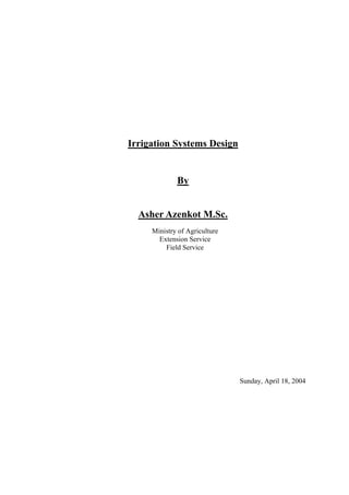
⇒ The sprinkler pressure along the lateral pipe declines faster along the first 40%
of the length than afterwards, fig 1.
⇒ The sprinkler flow rate along the lateral pipe declines faster along the first 40%
of the length than after, fig 2.
• The location of the sprinkler (or emitter) with the average pressure and flow rate
is 40% away from the lateral’s inlet.
⇒ Three quarters of the lateral head loss takes place along the first two fifth
sections (40%), fig. 1.
Fig. 1: The pressure reduction along 3" lateral pipe (156 m long) with Naan 233
sprinklers at 12 m apart.
0 12 24 36 48 60 72 84 96 108 120 132 144 156
20
40
60
80
100
120
Sprinklerpressurem
0
20
40
60
80
100
120
%ofheadloss
pressure (m) Pres Red % of reduction Plain line
pressure (m) 40 38.5 37.2 36.1 35.2 34.4 33.9 33.4 33 32.8 32.6 32.5 32.5 32.5
Pres Red 100 96 93 90 88 86 85 84 83 82 82 81 81 81
% of reduction 0 20 37 52 64 75 81 88 93 96 99 100 100 100
% of length 0 8 15 23 31 38 46 54 62 69 77 85 92 100
Plain line 100 96 92 88 84 80 76 72 68 64 60 56 52 48
27
29. Calculating the Head Loss Along lateral Pipe
⇒ The required sprinkler with Hs (pressure), qs (flow rate) and sl (space) is
selected from a catalogue.
⇒ The number of sprinkler (n) along the lateral is determined by (
L
Sl
).
⇒ The discharge rate at the lateral inlet is determined by (Qu = n x qs).
⇒ The lateral diameter (D) should be comply with a maximum of 20% head
loss along the pipe.
⇒ The head loss along the lateral (Qu, D and L) is computed by:
◊ assuming the lateral pipe is plain (without sprinklers), and
◊ The outcome is multiplied by F factor.
29
30. Example:
A flat field, 360 x 360 m, is irrigated with a hand moved aluminum lateral pipe (C = 140).
The water source to the lateral pipe is from a submain, which crosses the center of the field.
The selected sprinklers are Naan 233/92 with a nozzle of 4.5 mm, pressure of (hs) and flow
rate (qs ) of 1.44 m3
/hr. The space between the sprinklers is 12 meters apart, and the location
of the first sprinkler is 6 meters away from lateral inlet. The riser height is 0.8 meter and the
diameter is 3/4".
Answer
Lateral
360 m
Submain
The number of sprinklers on the lateral pipe is as follows:
sprinklersn 15
12
180
==
The length of the lateral pipe (l) is as follows:
l = (14 sprinklers x 12 m length) + 6 m = 174 meters
The flow rate of the lateral pipe is as follows:
Quu = 15 (sprinklers) x 1.44 m3/h = 21.6 m3/h
30
31. The maximum allowed head loss (20%) throughout the field is as follows:
∆h m= ⊗ =
20
100
25 5 eters
For a 2" aluminum pipe - the hydraulic gradient, which can be calculated from either a table
or a slide ruler or the Hazen-Williams equation, is: J = 188.9 ‰
The head loss in 2" plain aluminum pipe is as follows:
m
LJ
h
L
h
J 9.32
000,1
1749.188
000,1
000,1 =
⊗
=
⊗
=∆⇒⊗
∆
=
The F factor for 15 sprinklers is F15 = 0.363
mm
mFhhf
59.11
9.11363.09.3215
>
=⊗=⊗∆=∆
11.9 m is higher than 5 m. Therefore a larger pipe is taken.
For a 3" aluminum pipe - the hydraulic gradient calculated from a table or a monograph or a
slide ruler or the Hazen-Williams equation is: J = 26.2 ‰.
The head loss of a 3" plain aluminum pipe is as follows:
meters
LJ
h 6.4
000,1
1742.26
000,1
=
⊗
=
⊗
=∆
The F factor for 15 sprinklers is: F15 = 0.363
m
metersFhhf
566.1
66.1363.06.415
<
=⊗=⊗∆=∆
The difference of 5 - 1.66 = 3.34 meters head loss is kept for the submain head loss.
31
32. A Lateral Inlet Pressure
The pressure head at the lateral inlet (hu) is determined by:
riserhhh fsu +⊗+=
4
3
hu = lateral inlet pressure head
hs = pressure head of selected sprinkler
hf = head loss along lateral
riser = the height of the riser
Example:
Following the previous example, what is the inlet pressure?
hf = 1.66 meters
Riser height = 0.8 meters
hs = 25 meters
atmospheremh
riserhhh
u
fsu
7.2278.066.1
4
3
25
4
3
⇒=+⊗+=
+⊗=
32
33. A Lateral Laid out on a Slope
Once a lateral is laid out along a slope with an elevation difference of ∆Z meters between
the two ends, (hu ), then the pressure requirement at the lateral inlet is calculated as follows:
h h h riser
z
u s f= + ⊗ + ±
3
4 2
∆
hu = the lateral inlet pressure
hs = pressure head of selected sprinkler
hf = head loss along lateral
riser = riser height
+
∆Z
2
- adjustment for upward slope
−
∆Z
2
- adjustment for downward slope
Example:
Following the previous example, but this time with: a. 2% downward slope, or b. 2%
upward slope.
The difference elevation between the two ends is as follows:
± = ⊗ = ±∆Z m174
2
100
348. eters
a. 2% downward slope
mh
z
riserhhh
u
fsu
3.25
2
48.3
8.066.1
4
3
25
24
3
=−+⊗+=
∆
−+⊗+=
33
34. The pressure by the last sprinkler is as follows:
m
Zhh fu
12.2748.366.13.25 =+−
∆+−
The head loss between lateral inlet and last sprinkler is as follows:
m82.112.273.25 −=−
-1.82 meters is < than 5 meters, and the difference head loss of 5 meters (20%) is kept for
the submain head loss.
All the “20% head loss” is taken place along the submain pipe.Therefore, the pressure at the
inlet pipe to the field is 30.3 m.
b. 2% upward slope
mh
z
riserhhh
u
fsu
78.28
2
48.3
8.066.1
4
3
25
24
3
=++⊗+=
∆
−+⊗+=
The total head loss throughout the lateral pipe is as follows:
metershd 14.548.366.1 =+=∆ ≈ 5 meters
5.14 meters are just the permitted 20% head loss. Therefore, nothing is left for the submain.
In this case, pressure regulators should be installed in each lateral inlet.
34
35. "The 20% Rule"
In order to maintain up to 10% difference in flow rate between sprinklers or emitters within
a plot, then the pressure difference inside the plot should be up to 20%. This rule is carried
out only when the value of the exponent is 0.5 (see later).
The relationship between pressure and flow rate out of a sprinkler is as follows:
HgACQ ⊗⊗⊗⊗= 2
or Q x
HK ⊗=
Q - flow rate
C, K - constants depend on a nozzle or emitter type.
A - cross section area of a nozzle
H - pressure head
x (exponent) – the exponent depends on the flow pattern inside a nozzle. Usually, the
exponent value for a sprinkler is equal to 0.5. While the exponent value for emitters
depend on the flow pattern. The exponent is equal to 0 for an emitter with a flow or
pressure regulator, while for turbulence flow type (labyrinth emitter) is equal to 0.5, and
for hydro-cyclone pattern or very low flow rate is less than 0.5 and for a laminar flow
pattern is almost 1.0.
Unfortunately, most of the drip catalogues don't provide the exponent value, but describes
by a graph the relationship between pressure and flow discharge of different emitters. In this
case, to calculate the constants (K and x) by the previous equations are needed a few points
on the curve depicting the relation flow pressure of an emitter.
Example:
What is the expected difference discharge between two ends of the lateral sprinkler? When
the hydraulic gradient along a lateral pipe is 20%.
The flow rate of a sprinkler is as follows:
Q K H= ⊗ 0 5.
The relationship between two identical sprinklers which have a same constant K, and 20%
pressure difference is as follows:
%9089.08.0
8.0
)%20(8.0
1
1
1
1
2
12
1
2
1
2
1
2
5.0
1
5.0
22
≈===
⊗=
==
⊗
⊗
=
H
H
Q
Q
differenceHH
H
H
H
H
Q
Q
HK
HK
Q
Q
35
36. The difference in flow rate between the two ends is 10% (within “20% rule”), once the
exponent is equal to 0.5.
Example for micro-sprinklers:
A polyethylene lateral pipe, grade 4, has 10 micro-sprinklers at 10 meters apart, while the first
micro spinkler is stand only one half way. The flow rate of the selected sprinkler is qs = 120
l/h at hs = 20 meters. The riser’s height is 0.15 meter (can be ignored). What is the required
diameter of the lateral pipe?
n = 10 micro-sprinklers
Length = (9 sprinkler x 10 m) + 5 m = 95 meters
F10 = 0.384
Q mu =
⊗
=
10 120
1 000
12 3
,
. / h
The maximum allowable in the entire plot is =∆h
20
100
20 4⊗ = meters
The hydraulic gradient out of a slide ruler, monograph or Darcy-Weisbach equation for a 20
mm polyethylene pipe and Q = 1.2 m3
/h is J = 18.5%.
mh
Fhh
mh
f
f
74.6384.05.17
5.17
100
95
5.18
10
=⊗=∆
⊗∆=∆
=⊗=∆
6.74 meters head loss exceeds the allowable 4 meters (20%), therefore, a larger pipe is
tested.
The hydraulic gradient which can be found out from a slide ruler, monograph or Darcy-
Weisbach equation for 25 mm P.E. pipe and Q = 1.2 m3
/h is J = 5.8%.
mh
mh
f 1.2384.05.5
5.5
100
95
8.5
=⊗=∆
=⊗=∆
The head loss of 2.1 meters is less than the allowable 4 m (20%). The pressure difference
between the maximum allowed head loss and the actual head loss along the lateral (4 m - 2.1
m = 1.9 m) is the maximum head loss along the manifold (if pressure regulators are not in
used).
36
37. The required pressure by the lateral pipe inlet is as follows:
metershu 5.211.2
4
3
20 =⊗+=
37
38. Three Alternatives in Designing the Irrigation System
There are three general options for designing an irrigation system:
⇒ Option 1 - The rule of 20% is applied to all the sprinklers on the same subplot.
Any excess pressure over 20% between the subplots is controlled by flow or
pressure regulators.
⇒ Option 2 - The rule of 20% is applied to a single lateral pipe, and pressure
regulators control the pressure difference between the laterals. (It is common
in drip systems.)
⇒ Option 3 - The difference pressure along a lateral pipe exceeds the 20% head
loss by any desired amount (up to the value that the pipes and connectors can
stand). Therefore, flow or pressure regulators are used in each emitter or
sprinkler to control the excess pressure or flow. (It enables the use of longer
laterals or smaller diameter pipes than permitted by Option 1 or 2.)
38
39. Example:
Ten micro-sprinklers are installed along a plastic lateral pipe (grade 4) at 10 meters (32.8 ft.)
apart. (The first sprinkler is stand at 5 meters away from the inlet). The flow rate of the
selected sprinkler is qs = 120 l/h (0.5 GPM) at pressure of hs = 20 meters. The riser height is
0.15 meter (which can be ignored). What is the appropriate lateral pipe diameter and length, if
the field is designed and abided by options 1, 2 and 3?
n = 10, L = (9 ⊗10 + 5) = 95 m F10 = 0.384 Q m= hr
⊗
=
10 120
1 000
1 2 3
,
.. /
Option 1:
For a 20 mm polyethylene pipe - the hydraulic gradient which can be found out of a slide
ruler, monograph or Darcy-Weisbach equation for flow rate of Q = 1.2 m3
/h and 20 mm P.E.
pipe is J = 18.5%.
mFhh
mh
72.6384.05.17
5.17
100
95
5.18
10 =⊗=⊗∆=∆
=⊗=∆
Head loss of 6.72 meters exceeds the allowable 4 meters (20%). Therefore, a larger pipe is
tested.
For a 25 mm pipe - the hydraulic gradient taken out of a slide ruler, monograph or Darcy-
Weisbach equation for flow rate of Q = 1.2 m3
/h and 25 mm P.E. pipe is J = 5.8%.
mFhh
mh
11.2384.05.5
5.5
100
95
8.5
10 =⊗=⊗∆=∆
=⊗=∆
The head loss difference 4 m - 2.11 m = 1.89 meters is available for the manifold head
loss.
The inlet lateral pressure is as follows:
atmospheremetershu 15.258.2111.2
4
3
20 ⇒=⊗+=
39
40. Option 2:
If the allowable pressure variation along the lateral pipe is 4 meters, then 25 mm P.E. pipe is
too much and 20 mm too small. Therefore, to overcome a head loss greater than 20% either a
combination of two diameter pips can be used, or pressure regulators can install in every
lateral inlet.
The design procedure for the combined lateral (two different diameters) pipes is as follows:
⇒ Try first a 25 mm diameter pipe along 35 meters (n = 4) and a 20 mm diameter
pipe along 60 meters (n = 6). The head loss calculation is as follows:
◊ The head loss for a 25 mm diameter pipe along 95 m, n = 10 and Q = 1.2
m3
/h is calculated as previously done, which was 2.11 m, then,
e. The head loss for 25 mm diameter pipe along 60 m, n = 6 and F6 = 0.458 is
calculated as follows:
The flow rate is: Q m= hr
⊗
=
6 120
1 000
0 72 3
,
. /
The hydraulic gradient taken out of a table, a slide ruler or Darcy-Weisbach
equation for 25 mm diameter pipe with a flow rate of 0.72 is J = 2.4%.
Therefore, the head loss for 60 meters lateral is as follows:
64.0458.04.1
4.1
100
60
4.2
6 =⊗=⊗∆=∆
=⊗=∆
Fhh
mh
f
The head loss for 25 mm diameter pipe along 35 meters with four sprinklers is as follows:
2.11 m - 0.64 = 1.47 meters
40
41. ◊ The head loss for 20 mm diameter pipe along 60 meters with n = 6 and F6 =
0.458 is calculated as follows:
The flow rate is: Q m= hr
⊗
=
6 120
1 000
0 72 3
,
. /
f. The hydraulic gradient taken out of a table, a slide ruler or Darcy-Weisbach
equation for 25 mm diameter pipe with a flow rate of 0.72 is J = 7.6%.
Therefore, the head loss for 60 meters lateral is as follows:
mFhh
mh
f 06.2458.05.4
5.4
100
60
6.7
6 =⊗=⊗∆=∆
=⊗=∆
The total head loss along the combined lateral pipe with 25 and 20 mm diameter is as
follows:
mhhhf 53.306.247.12025 =+=∆+∆=∆
⇒ Since the total (3.5 m) is less than 4.0 meters. Therefore, it is possible to
retry a shorter 25 mm pipe with a length of 25 meters and n = 3 and a longer
20 mm diameter pipe along 70 meters and n = 7. The previous ways of
calculation should be repeated over. The new head loss
∆hf
∆hf is 4.5 meters,
which exceeds the limit of 4 meters - (20% rule). Therefore, the first choice is
taken.
⇒ The inlet pressure requirement by the last lateral is as follows:
h m m atmosphereu = + ⊗ = ≈ ⇒20
3
4
35 22 7 23 2 3. . .
41
42. Option 3:
The lateral pipe is designed either with flow or pressure regulators in every micro-sprinkler.
The lateral diameter can be reduced to 20 mm or even further to 16 mm, unless the inlet
pressure is less than the pipe and connectors can stand. (The reduced cost for the pipe must be
less than the additional cost for the energy due to a higher pressure and for regulators).
In case of 20 mm diameter, the head loss ( ∆hf ) is 6.72 meters (see Option 1). Therefore, the
pressure requirement at the inlet of the last lateral pipe is:
.7.22772.2672.620 atmmhu ⇒≈=+=
In case of option 3, the entire head loss along a lateral pipe is added to the lateral inlet
pressure. The maximum inlet pressure should be complied with the pipe grade.
42
43. Example (on a slope):
A manifold was installed along the center of a rectangular field. The lateral pipes were
hooked up to the two sides of the manifold pipe. The difference in elevation between the
center and the end of the field is 2 meters (either positive or negative). Each lateral pipe has
eight 120 l/hr micro-sprinklers at 6 meters apart and the pressure (hs) is 25 meters. What is the
required diameter of the lateral pipes if the system is designed and abides by option 1?
Answer
The laterals’ head loss along the two sides of the manifold should be close enough (in a way
that the total head loss due to the difference in elevation and friction head loss on both sides
of the manifold should be almost the same).
The maximum head loss between the sprinklers throughout the field (first and last) is
20
100
25 5⊗ = meters (20% rule).
Let try a 20 mm lateral pipe on the two sides:
n = 8 F8 = 0.394 L = (7 sprinklers x 6 m) + 3 m = 45 m
Q m= ⊗ =8
120
1 000
0 96 3
,
. / hr
The hydraulic gradient for Q = 0.96 m3
/hr and D = 20 mm is J = 12.2%
21.2394.062.5
62.5
100
45
5.12
=⊗=∆
=⊗=∆
fh
mh
The laterals’ head loss on the downward side is as follows:
.56.26.25
2
2
21.2
4
3
25 atmhu ⇒=−⊗⊕=
The pressure by the last sprinkler is as follows:
atmospheremh 5.24.25221.26.258 ⇒=+−=
43
44. Therefore, the pressure difference between the two ends is as follows:
.02.02.04.256.258 atmhhh ud ⇒=−=−=
The laterals’ head loss on the upward slope side is as follows:
The pressure in the lateral inlet is as follows:
.76.265.27
2
2
21.2
4
3
25 atmhu ⇒=+⊗⊕=
The pressure at the last sprinkler is as follows:
.3.24.23221.265.278 atmh ⇒=−−=
(The pressure head loss along the upward lateral is 27.65 m - 23.4 m = 4.25 m, which is
less than 5 m - 20% rule)
The pressure requirement for the upward laterals is 27.65 meters and for the downward
laterals is only 25.6 meters. The head loss along the upward laterals is 4.25 meters, almost all
the permitted 20% (5 m). Therefore, the manifold’s size should be increased or pressure
regulators should be installed in the lateral inlets, or the upward lateral will be increased to 25
mm, or the manifold can be relocated at a higher point. (The aim is to reduce the difference
pressure between the inlet pressure to both sides laterals to nill).
When 20 mm lateral pipes are in use, the values of hu for both sides of the manifold vary by
27.65 - 25.6 = 2.05 m
To avoid this difference (hu) in the inlet pressure, the upward 20 mm laterals can be replaced
by 25 mm. The inlet head (hu) for 25 mm is 26.5 m. Therefore, the difference inlet pressure
for both sides of the manifold will be less, only 26.5 - 25.7 = 0.8 m.
More economical alternative is by relocating the manifold away from center of the field to a
higher elevation. That way, 6 sprinklers will be on each upward laterals side and 10 sprinklers
on the downward laterals sides (trial and error).
Downward laterals:
The head loss for:
D = 20 mm n = 10 L = (9 sprinkler x 6 m) + 3 m = 57 m
Q = 1.2 m3
/hr F10 = 0.384 from monograph is J = 18.5%, therefore for the lateral the head
loss is as follows:
44
45. mmFhh
mh
f 2.415.4384.053.10
53.10
100
57
5.18
10 ≈=⊗=⊗∆=∆
=⊗=∆
The slope is m28.2
100
57
44.4%44.4
45
2
=⊗⇒=
The pressure at the lateral inlet is as follows:
mhu 1.27
2
28.2
2.4
4
3
25 =−⊗+=
The pressure head by the last lateral sprinkler is as follows:
mZhhh fud 2.2528.22.41.27 =+−=∆+−=
The head loss along the downward lateral is as follows:
mhhh du 9.12.251.27 =−=−=∆
Upward laterals:
The head loss from a slide ruler for n = 6 F6 = 0.405 L = (5 sprinklers x 6) + 3 = 33 m Q
= 7.2 m3
/hr is J = 7.6%
mmFhh
mh
f 101.1405.05.2
5.2
100
33
6.7
6 ≈=⊗=⊗∆=∆
=⊗=∆
The elevation difference is m32.1
100
33
0.4 =⊗ for a slope of 4%.
The pressure head at the lateral inlet is as follows:
m
Z
hhh fsu 51.26
2
32.1
0.1
4
3
25
24
3
=+⊗+=
∆
+⊗+=
The pressure head at the last lateral sprinkler is
mZhhh fud 19.2432.10.151.26 =−−=∆−∆−=
45
46. mhhh du 32.219.2451.26 =−=−=∆
The values of hu for both sides 27.1 m and 26.51 m are practically the same. The maximum
tolal head loss along the laterl pipe is is 2.3 m, therefore, 2.7 meters are available as a head
loss for the manifold.
∆h
46
47. Design of a Manifold
The manifold is a pipe with multiple outlets (similar to lateral pipe); therefore, the manifold
designed procedure is the same way as it is done for a lateral. The size of a plot and the
number of subplots in each field depends on (the way the field is divided), irrigation rate, crop
water requirement, and the number of shifts and etc.
Distribution of pressure head and water in a subplot
Example:
A fruit tree plot is designed for irrigation with a solid set system. A manifold is laid
throughout the center of the field. The whole plot is irrigated simultaneously (one shift). The
flow rate of the selected micro-sprinkler is qs = 0.11 m3
/hr at a pressure (hs) of 2.0
atmospheres. The space between the micro-sprinklers along the lateral is 8 meters (20 ft.) and
6 meters (19.7 ft.) between the laterals. What is the required diameter of the pipes? (The local
head loss is 10% of the total head loss and is taken in account.)
Answer
8 x 6 m lateral
96 m manifold
The maximum allowable pressure head difference is 20
20
100
4⊗ = meters.
The number of micro-sprinkler on each lateral is
48
8
6=
F6= 0.405 L = (5 sprinklers x 8 m) + 4 m = 44 m
Lateral flow rate is: Q = 0.11 m3
/hr x 6 sprinklers = 0.66 m3
/hr
The hydraulic gradient for 16 mm P.E. pipe with a flow rate of Q = 0.66 m3
/hr is J = 22.3%
47
48. mh 8.9
100
44
3.22 =⊗=∆
The head loss in 16-mm lateral pipe (including 10% local head loss) is as follows:
∆hf = (10% local head loss) x ∆h x F6 = 1.1 x 9.8 x 0.405 = 4.36 m
4.36 m head loss exceeds the allowable 4-meter (20%). So we have to try the head loss for
20-mm P.E. lateral pipe.
The hydraulic gradient for 20 mm P.E. pipe and Q = 0.66 m3
/hr is J = 6.5%.
mh 86.2
100
44
5.6 =⊗=∆
The head loss in 20-mm lateral pipe (including 10 local head loss) is as follows:
∆h mf = ⊗ ⊗ =11 2 8 0 405 13. . . .
1.3 m head loss is less than 4 m (20%). Therefore this pipe can be selected as a lateral.
The lateral inlet pressure is as follows:
h h hu s f= + ⊗ = + ⊗ =
3
4
20
3
4
13 21∆ . m
m
The water pressure at the last micro-sprinkler on the lateral is as follows:
h h hu f6 21 13 19 7= − = − =∆ . .
Manifold Design:
The number of lateral pipes is ( ) ( )N two sides= ⊗ − =
96
6
2 32
The length of the manifold pipe is as follows:
L = (31 laterals x 6 m) + 3 = 93 m
The flow rate is as follows:
Q = 32 x 0.66 = 21.1 m3
/hr
48
49. The hydraulic gradient for 63 mm P.E. pipe with 32 outlets (F32 = 0.376) and Q = 21.1 m3
/hr
is J = 7.2%.
The head loss along the manifold pipe is as follows:
mh 69.6
100
93
2.7 =⊗=∆
The manifold's pressure head loss (63-mm P.E. pipe, including 10% due to local head loss)
is as follows:
mFhlossheadlocalhf 76.2376.069.61.1)%10( 32 =⊗⊗=⊗∆⊗=∆
The inlet pressure of the water at the manifold is as follows:
m
Z
hhh fulum 07.2376.2
4
3
21
24
3
=⊗+=
∆
±∆⊗+=∆
The inlet pressure by the last lateral is as follows:
mhhh fumd 31.2096.207.23 =−=∆−=∆
The maximum pressure throughout the plot is at the first lateral inlet, which is 23.2 meters
(2.3 atmosphere).
The minimum pressure throughout the system is at the last sprinkler on the last lateral,
which is as follows:
20.31 - 1.3 = 19.01 m
The pressure difference between the first and last sprinkler is as follows:
23.07 - 19.01 = 4.06 m (i.e. just almost 4 meters (20%))
49
50. Design of Irrigation System
The sequence for designing an irrigation system is as follows:
a. Taking in considerations: soil, topography, water supply and quality, type of
crops.
b. Taking in considerations: farm schedule.
c. Estimate water application depth at each irrigation cycle.
d. Determine the peak period of daily water consumption.
e. Determine the frequency of water supply.
f. Determine the optimum water application rate.
g. Taking in considerations several alternative of irrigation system types.
h. Determine the sprinklers or emitters spacing, discharge, nozzle sizes, water
pressure.
i. Determine the minimum number of sprinklers or emitters (or a size of subplot)
which must be operated simultaneously.
j. Divide the field into sub-plots according to the crops, availability of water and
number of shifts.
k. Determine the best layout of main and laterals.
l. Determine the required lateral size.
m. Determine the size of a main pipe.
n. Select a pump.
o. Prepare plans, schedules, and instructions for proper layout and operation.
p. Prepare a schematic diagram for each set of submains or manifolds, which can
operate simultaneously.
q. Prepare a diagram to show the discharge, pressure requirement, elevation and
pipe length.
r. Select appropriate pipes, starting at the downstream end and ending up by the
water source.
50
51. Appendix 1: Unit conversion
Length:
1 inch 2.54 cm
1 ft. 30.5 cm
1 m 100 cm
1 m 3.281 ft.
1 m 39.37 inches
1 cm 10 mm
1 km 1,000 m
Area:
1 sq.m 10.76 sq ft.
1 acre 4048 sq m
1 ha 10,000 sq. m
1 ha 2.47 acre
Weight:
1 lb 0.454 kg
1 kg 2.205 lb
1 kg 1,000 gr
1 oz 29 gr
Volume:
1 gal (USA) 3.78 li
1 Imperial gal 4.55 li
1 m3 1,000 li
1 m3 220 Imperial gal
Pressure
1 atmosphere (at) 1 kg/cm2
1 psi 1 lb/inch2
1 at 14.22 psi
10 m 1 at
51