Social Cost

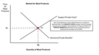
1. Price
Of
Meat
Products
Quantity of Meat Products
Demand (Private Benefit)*
Supply (Private Cost)*
Pe
Qe
Market for Meat Products
“A”
Here is the Market for various Meat Products in equilibrium.
Note that ONLY the PRIVATE COSTS (Supply Curve) of societal
resources are included in the production of meat and ONLY the
PRIVATE BENEFITS (Demand Curve) of consuming those
resources are included in the PRICE.

2. Price
Of
Meat
Products
Quantity of Meat Products
Demand (Private Benefit)*
Supply (Private Cost)*
Pe
Qe
Market for Meat Products
“A”
Q S.O.
(Socially Optimal)
The article suggests that there is too much production of meat
products which leads to damage to the environment. The more
“Socially Optimal” level of production (“Q s.o.”) is something
LESS that the Private Market quantity of “Qe” denoted by the
dotted BLUE line.

3. Price
Of
Meat
Products
Quantity of Meat Products
Demand (Private Benefit)*
Supply (Private Cost)*
Pe
Qe
Market for Meat Products
“A”
“C”
Q S.O.
(Socially Optimal)
“B” Note at “Q s.o.” the market is not in equilibrium. It is at Point
“B” along Demand (Private Benefit) and Point “C” along Supply
(Private Cost).
To get back to equilibrium we need to do one of two things:
Shift the Supply Curve (Private Cost) to the LEFT or Shift
Demand Curve (Private Benefit) to the LEFT.
The end goal is to “internalize” into Private Market
transactions the external costs meat products impose on
the environment that producers and consumers are
presumably not paying for.

4. Price
Of
Meat
Products
Quantity of Meat Products
Demand (Private Benefit)*
Supply (Private Cost)*
Pe
Qe
Market for Meat Products
“A”
“C”
Q S.O.
(Socially Optimal)
“B”
Let’s first look at Internalizing the cost of environmental
damage on the Producer of Meat Products.
This can be accomplished by imposing a TAX on the
PRODUCTION of Meat Products (“supply side”). The tax
represents societies attempt at recovering some/all the
additional costs associated with the production of meat
products….

5. Price
Of
Meat
Products
Quantity of Meat Products
Demand (Private Benefit)*
Supply (Private Cost)*
Pe
Qe
Market for Meat Products
“A”
“C”
Q S.O.
(Socially Optimal)
Internalizing the “Social Cost” will increase the cost of
producing Qe at Point “A” by “Pe + the Tax” along
Supply (Private Cost)* to Point “D”.
“D”
“B”

6. Price
Of
Meat
Products
Quantity of Meat Products
Demand (Private Benefit)*
Supply (Private Cost)*
Pe
Qe
Market for Meat Products
“A”
“B”
“C”
Q S.O.
(Socially Optimal)
Supply (Private Cost + Social Cost)
“D”
Ceterus Paribus, what is true from Point “A” to Point “B”
is going to be true for EVERY OTHER point along Supply
(Private Cost)*--- for example Point “C” to Point “B”.
The NEW Market Supply Curve, “Supply (Private Cost +
Social Cost), NOW includes the tax that is designed to
impose/compensate society for the Externality.

7. Price
Of
Meat
Products
Quantity of Meat Products
Demand (Private Benefit)*
Supply (Private Cost)*
Pe
Qe
Market for Meat Products
“A”
“B”
“C”
Q S.O.
(Socially Optimal)
Supply (Private Cost + Social Cost)
“D”
Here is an important takeaway: The Supply Curve
(Private Cost)* represents “what is” in the marketplace
and Supply Curve (Private Cost +Social Cost)
represents “should be”.
The DIFFERENCE (in math terms) between Equilibrium
Point “A” and “B” is that “B” now includes the cost of
the Externality up to Point “D”....

8. Price
Of
Meat
Products
Quantity of Meat Products
Demand (Private Benefit)*
Supply (Private Cost)*
Pe
Qe
Market for Meat Products
“A”
“B”
“C”
Q S.O.
(Socially Optimal)
Supply (Private Cost + Social Cost)
“D”
...the Triangle formed by “A”, “B” and “D” represents
the area of “DEADWEIGHT LOSS”---the production and
pricing of Meat Products that do not cover the TRUE
COST to society for that production.
The Marginal Cost (between Points “B” and “D” is
GREATER THAN the Marginal Benefit (between Points
“B” and “A”)
“DWL”

9. Price
Of
Meat
Products
Quantity of Meat Products
Demand (Private Benefit)*
Supply (Private Cost)*
Pe
Qe
Market for Meat Products
“A”
“B”
“C”
Q S.O.
(Socially Optimal)
Supply (Private Cost + Social Cost)
“D”
Double Check:
Pick ANY Market quantity/point between “Q s.o.” and “Qe” along the
x-axis.
Draw a straight line up to where it hits the “Supply(Private + Social
Cost)” Curve. Note that the line cuts through the Demand Curve
BELOW the point where it cuts the Supply Curve---The Social Cost of
this quantity is GREATER than the Private Benefit the consumer
receives: Deadweight Loss!
“DWL”