5. Chapter 1
Hyperbolic PDEs
We consider the hyperbolic equation
ut + aux = 0
for t ≥ 0 and initial condition u(0, x) = u0 (x). The unique solution to this problem is given by
u(t, x) = u0 (x − at),
i.e., the solution is wave traveling right if a > 0 and left if a < 0.
We will show (a) how to generate schemes for its numerical solution, (b) verify that these schemes are
a good approximation to the differential equation (i.e., are consistent) and (c) that the numerical solution
converges to the solution to the differential equation.
The idea in using finite differences to solve a PDE is to select a grid in time and space (with meshlengths
k and h, respectively) and to approximate the values u(mk, nh) for integer m, n. All all that follows u will
denote the exact solution to the PDE and
(time) n
v(space) = vm ≈ u(mh, kn)
will denote the approximate finite difference solution.
We will approximate derivatives of a function f as follows:
f (x + h) − f (x)
δ+ f (x) = forward difference
h
f (x) − f (x − h)
δ− f (x) = backward difference
h
f (x + h) − f (x − h)
δ0 f (x) = centered difference
2h
For a grid function v = (. . . , v−2 , v−1 , v0 , v1 , v2 , . . .) we have:
vm+1 − vm
δ+ vm = forward difference
h
vm − vm−1
δ− vm = backward difference
h
vm+1 − vm−1
δ0 vm = centered difference
2h
1.1 Consistency, Stability, Well-posedness, and Convergence
Definition 1 (Consistency). We say that a finite difference scheme Pk,h v = f is consistent with the PDE
P u = f of order (r, s) if for any smooth function φ
P φ − Pk,h φ = O(k r , hs ) (1.1)
5
6. 6 CHAPTER 1. HYPERBOLIC PDES
To verify consistency expand φ in Taylor series and make sure (1.1) holds.
Definition 2 (L2 norm). For a function w = (. . . , w−2 , w−1 , w0 , w1 , w2 , . . .) on a grid with step size h:
∞ 1/2
2
w = h |wm |
m=−∞
For a function f on the real line:
∞ 1/2
f = |f (x)|2 dx
−∞
n
Definition 3 (Stability). A finite one-step difference scheme Pk,h vm = 0 for a first-order PDE is stable if
there exist numbers k0 > 0 and h0 > 0 such that for any T > 0 there exists a constant CT such that
v n ≤ CT v 0
for 0 ≤ nk ≤ T, 0 < h ≤ h0 , 0 < k ≤ k0 .
Definition 4 (Well-posedness). The initial value problem for the first-order PDE P u = 0 is well-posed if
for any time T ≥ 0, there is a constant CT , such that any solution u(t, x) satisfies
u(t, x) ≤ CT u(0, x) , for 0 ≤ t ≤ T.
Definition 5 (Convergence). A one-step finite difference scheme approximating a PDE is convergent if for
n 0
any solution to the PDE, u(t, x), and solution to the finite difference scheme vm , such that vm → u(0, x) as
n
mh → x, we have vm → u(t, x) as (nk, mh) → (t, x) (as h, k → 0).
Theorem 1 (Lax). A consistent finite difference scheme for a PDE for which the initial value problem is
well-posed is convergent if and only if it is stable.
Theorem 2 (The Courant–Friedrichs–Lewy Condition). A necessary condition for stability of the explicit
scheme for the hyperbolic equation ut + aux = 0:
n+1 n n n
vm = αvm−1 + βvm + γvm+1
with k/h = λ held constant is
|aλ| ≤ 1.
n
Proof. The solution is u(t, x) = u0 (x − at) and u(1, 0) = u0 (−a). The finite difference scheme v0 depends
0
only on vm for |m| ≤ n. Therefore |hn| ≥ | − a|. Since kn = 1, we have n = 1/k and |n/k| ≥ |a| or
|aλ| ≤ 1.
1.2 Fourier Analysis
Fourier Transform and Inversion formula
• For u defined on R
∞ ∞
1 1
u(ω) = √
ˆ e−iωx u(x)dx, u(x) = √ eiωx u(ω)dω
ˆ
2π −∞ 2π −∞
• For a grid function v = (. . . , v−2 , v−1 , v0 , v1 , v2 , . . .) with grid spacing h (here ξ ∈ [−π/h, π/h])
∞ π/h
1 1
v (ξ) = √
ˆ e−imhξ vm h, vm = √ eimhξ v (ξ)dξ
ˆ
2π m=−∞
2π −π/h
Theorem 3 (Parseval).
u(x) = u(ω) ,
ˆ v = v .
ˆ
2 π/h
(where v
ˆ = −π/h
|ˆ(ξ)|2 dξ.)
v
7. 1.3. VON NEUMANN ANALYSIS 7
1.3 Von Neumann Analysis
Provides an uniform way of verifying if a finite difference scheme is stable.
Example 1. Let’s study the forward-time backward-space scheme
n+1 n
vm − vm v n − vm−1
n
+a m = 0.
k h
Rewrite as
n+1 n n
vm = (1 − aλ)vm + aλvm−1 ,
where λ = k/h. Use the Fourier inversion formula
π/h
n 1
vm = √ eimhξ v n (ξ)dξ
ˆ
2π −π/h
and substitute to obtain
π/h π/h
1 1
√ eimhξ v n+1 (ξ) dξ = √
ˆ eimhξ [(1 − aλ) + aλe−ihξ ]ˆn (ξ) dξ.
v
2π −π/h 2π −π/h
∗ ∗∗
The Fourier transform is unique, so (*) must equal (**):
v n+1 (ξ) = [(1 − aλ) + aλe−ihξ ]ˆn (ξ).
ˆ v
Denote g(hξ) ≡ (1 − aλ) + aλe−ihξ , called amplification factor. We have
n 0
v n (ξ) = g(hξ)ˆn−1 (ξ) = . . . = g(hξ)
ˆ v v (ξ).
ˆ
Now
π/h π/h
vn 2
= |ˆn (ξ)|2 dξ =
v |g(hξ)|2n |ˆ0 (ξ)|2 dξ.
v
−π/h −π/h
Therefore v n ≤ v 0 (i.e., the scheme is stable), if |g(hξ)| ≤ 1. Write θ = hξ and evaluate |g(θ)|2
|g(θ)|2 = |(1 − aλ) + aλe−ihξ |2
= (1 − aλ + aλ cos θ)2 + a2 λ2 sin2 θ
= (1 − 2aλ sin2 θ )2 + 4a2 λ2 sin2
2
θ
2 cos2 θ
2
= 1 − 4aλ(1 − aλ) sin2 θ .
2
Thus |g(θ)| ≤ 1 if 0 ≤ aλ ≤ 1. Then v n ≤ v 0 and the scheme is stable if 0 ≤ aλ ≤ 1.
Theorem 4 (Stability condition). A one-step finite difference scheme is stable if and only if there exist
positive constants K, h0 , k0 such that
|g(θ, k, h)| ≤ 1 + Kk
for all θ, 0 < k ≤ k0 , 0 < h ≤ h0 . If g is independent of k, then the condition is
|g(θ, k, h)| ≤ 1.
Proof. Assume g(θ, k, h) ≤ 1 + Kk for some K.
π/h π/h
vn 2
= |g|2n |ˆ0 (ξ)|2 dξ ≤ (1 + Kk)2n
v |ˆ0 (ξ)|2 dξ ≤ (1 + Kk)2n v 0
v 2
−π/h −π/h
8. 8 CHAPTER 1. HYPERBOLIC PDES
Now nk ≤ T and (1 + Kk)n ≤ (1 + Kk)T /k ≤ eKT , meaning v n ≤ eKT v 0 and the scheme is stable.
Conversely, assume that for any C there exists an interval [θ1 , θ2 ] such that |g| ≥ 1+Ck for θ ∈ [θ1 , θ2 ], h ∈
(0, h0 ], and k ∈ (0, k0 ]. Let
0 if hξ ∈ [θ1 , θ2 ],
v 0 (ξ) =
ˆ −1
h(θ2 − θ1 ) if hξ ∈ [θ1 , θ2 ].
Now v 0 = 1 and
ˆ
π/h θ2 /h
h 1
vn 2
= |g|2n |ˆ0 (ξ)|2 dξ =
v |g|2n dξ ≥ (1 + Ck)2n ≥ e2T C v 0 2
−π/h θ1 /h θ2 − θ1 2
for n near T /k. Therefore the scheme is unstable if C can be arbitrarily large. If g is independent of h and
k, then |g| ≤ 1 + Kk must hold for any 0 < k ≤ k0 , therefore |g| ≤ 1.
n
In practice to analyze a finite difference scheme we do not write integrals. Instead we replace vm by
n imθ
g e and solve for g.
Example 2. Forward-time centered space
n+1 n
vm − vm v n − vm−1
n
+ a m+1 = 0.
k 2h
g n+1 eimθ − g n eimθ g n ei(m+1)θ − g n eim−1θ g−1 eiθ − e−iθ
0= +a = g n eimθ +a .
k 2h k 2h
So g(θ) = 1 − iaλ sin θ, with λ = k/h. If λ is constant, then |g(θ)|2 = 1 + a2 λ2 sin2 θ > 1 and the scheme is
unstable.
Example 3. The Lax–Wendroff scheme:
n+1 n aλ n n a2 λ2 n n n
vm = vm − (vm+1 − vm−1 ) + (vm+1 − 2vm + vm−1 ),
2 2
so the amplification factor is:
aλ iθ a2 λ2 iθ
g(θ) = 1− (e − e−iθ ) + (e − 2 + e−iθ )
2 2
= 1 − iaλ sin θ − a2 λ2 (1 − cos θ)
= 1 − 2a2 λ2 sin2 θ
2 − iaλ sin θ
Thus
2
|g(θ)|2 = (1 − 2a2 λ2 sin2 θ )2 + 2aλ sin θ cos θ
2 2 2
= 1 − 4a2 λ2 (1 − a2 λ2 ) sin4 θ
2
The scheme is stable only when |g(θ)| ≤ 1, i.e., when |aλ| ≤ 1.
Example 4. For the Crank–Nicolson scheme
n+1 n aλ n+1 n+1 n n
vm = vm − (v − vm−1 + vm+1 − vm−1 )
4 m+1
we obtain
1 − 1 iaλ sin θ 1 + ( 1 aλ sin θ)2
g(θ) = 2
thus |g(θ)|2 = 2
=1
1 + 1 iaλ sin θ
2
1
1 + ( 2 aλ sin θ)2
so this scheme is unconditionally stable.
9. 1.4. THE LEAP-FROG SCHEME 9
1.4 The Leap-Frog Scheme
In this section we prove that Leap-frog is stable if and only if |aλ| < 1. The scheme is
n+1
vm − vm n−1 v n − vm−1
n
+ a m+1 = 0, i.e., n+1 n−1 n n
vm = vm + aλ(vm+1 − vm−1 ).
2k 2h
vm+1 −vm−1
Write δ0 vm = 2h . Then
n+1 n
vm −2kaδ0 1 vm
n = · n−1 .
vm 1 0 vm
Fourier transform for vectors = Fourier transform in each component:
n+1 π/h
vm 1 v n+1 (ξ)
ˆ
n = √ eimhξ dξ,
vm 2π −π/h v n (ξ)
ˆ
∞
v n+1 (ξ)
ˆ 1 n+1
vm
= √ e−imhξ h
v n (ξ)
ˆ 2π
n
vm
m=−∞
and Parseval for vectors (| · | means the 2-norm for vectors or matrices so we can tell it apart from the
L2 -norm)
2 ∞ 2 π/h 2 2
v n+1 n+1
vm v n+1 (ξ)
ˆ v n+1 (ξ)
ˆ
=h = dξ = .
vn n
vm −π/h v n (ξ)
ˆ v n (ξ)
ˆ
m=−∞
Now Fourier of Leap-Frog:
π/h π/h
1 v n+1 (ξ)
ˆ −2kaδ0 1 1 v n (ξ)
ˆ
√ eimhξ dξ = √ eimhξ dξ
2π −π/h v n (ξ)
ˆ 1 0 2π −π/h v n−1 (ξ)
ˆ
π/h
1 −2kaδ0 eimhξ v n (ξ) + eimhξ v n−1 (ξ)
ˆ ˆ
= √ dξ
2π −π/h eimhξ v n (ξ)
ˆ
π/h ihξ
−e−ihξ
1 −2ka e 1 v n (ξ)
ˆ
= √ eimhξ 2h dξ
2π −π/h 1 0 v n−1 (ξ)
ˆ
π/h
1 −2iaλ sin(hξ) 1 v n (ξ)
ˆ
= √ eimhξ dξ
2π −π/h 1 0 v n−1 (ξ)
ˆ
Therefore
v n+1 (ξ)
ˆ −2iaλ sin(hξ) 1 v n (ξ)
ˆ v n (ξ)
ˆ v 1 (ξ)
ˆ
= =G· = . . . = Gn · .
v n (ξ)
ˆ 1 0 v n−1 (ξ)
ˆ v n−1 (ξ)
ˆ v 0 (ξ)
ˆ
G(hξ)
10. 10 CHAPTER 1. HYPERBOLIC PDES
Parseval now gives
2 2
v n+1 v n+1 (ξ)
ˆ
=
vn v n (ξ)
ˆ
π/h 2
v 1 (ξ)
ˆ
= (G(hξ))n · dξ
−π/h v 0 (ξ)
ˆ
π/h 2
v 1 (ξ)
ˆ
≤ |G(hξ)|n · dξ
−π/h v 0 (ξ)
ˆ
2
v 1 (ξ)
ˆ
≤ max |G(hξ)|2n
|hξ|≤π v 0 (ξ)
ˆ
2
v1
= max |G(hξ)|2n .
|hξ|≤π v0
Remains to see when the 2-norm of G is bounded. Jordan form: G = T ΛT −1 and Gn = T Λn T −1 .
Characteristic polynomial:
g 2 + 2iaλ sin(hξ)g − 1 = 0
Λn bounded only if the roots (not to be confused with λ): |λ1,2 | ≤ 1, but λ1 λ2 = −1, so we must have
|λ1 | = |λ2 | = 1. Eigenvalues (denote s ≡ sin(hξ) for short):
λ1,2 = −iaλs ± 1 − (aλs)2 .
If |aλ| > 1, then there exists ξ, s.t. |aλs| > 1 and both λ1 and λ2 are purely imaginary and distinct, so one
of them will be > 1 and the other < 1 in magnitude. So we must have |aλ| ≤ 1.
When |aλ| ≤ 1 we have |λ1,2 |2 = (aλs)2 + 1 − (aλs)2 = 1. Therefore both λ1 and λ2 are on the unit circle.
If λ1 = λ2 , then Jordan form of G is (exercise):
−λ1 −1
1 1 λ1 λ2 1
G=
−λ2 −λ1 λ2 −λ1 + λ2
Exercise: |A| ≤ A F =( i,j |aij |2 )1/2 (Frobenius norm).
Now
√
n n −1 −1 −1
√ 4 2
|G | ≤ |T Λ T | ≤ |T | · 1 · |T |≤ T F T F ≤ 4· ≤
|−2 1− |aλ|2 | 1 − |aλ|2
is nicely bounded. Going back to Parseval
√
v n+1 2 v1
≤
vn (1 − |aλ|2 )1/4 v0
and Leap-frog is stable.
Next case: λ1 = λ2 . It occurs when sin(hξ) = ±1 and |aλ| = 1. Assume aλs = 1, (the −1 case is
analogous).
−2i 1 1 1 −i −i 0 −i
G= = = T ΛT −1
1 0 i 0 −i 1 i
A little unusual to write a Jordan block with −i in position (1, 2) but legal and, in this case, convenient.
n
1 1 1 n
Gn = T (−i)n T −1 = (−i)n T T −1 ,
0 1 0 1
11. 1.5. DISSIPATION 11
i.e., G(±π/2) will blow up. You’d think that there may be cancellation, but no:
1 n
n= = |in T −1 Gn T | ≤ |T | · |Gn | · |T |
0 1
and both |T | and |T −1 | are nicely bounded by (say) 2, so |Gn | ≥ n/4 = T /(4k) → ∞ as k → 0.
The stability condition is therefore |aλ| < 1.
1.5 Dissipation
We would expect the wave equation to propagate the initial condition with a constant speed a, including all
frequencies that make up that initial condition.
Unfortunately the discrete nature of our data means that instead of the initial condition u0 (x) we have
n
a discrete version of it—v0 .
The initial condition u0 (x) is a superposition (in theory) of an infinite number of frequencies (think
n
Fourier expansion), whereas v0 only inherits the frequencies ξ ∈ [−π/h, π/h]. All higher frequencies are
ignored by our discrete initial condition. Recall that the Fourier transform v n (ξ) of v n is only defined for
ˆ
ξ ∈ [−π/h, π/h].
Obviously different frequencies are treated differently and we would like to get a better understanding of
that treatment. Example is the best way to go here. Consider Lax–Friedrichs:
vm − 1 (vm+1 + vm−1 )
n+1 n n n
v n − vm−1
2
+ a m+1 = 0,
k 2h
equivalently,
n+1 1−aλ n 1+aλ n
vm = 2 vm+1 + 2 vm−1 .
Von Neumann analysis implies
g(hξ) = cos(hξ) − iaλ sin(hξ),
|g(hξ)|2 = cos2 (hξ) + (aλ)2 sin2 (hξ).
Let θ = hξ as usual.
We see that θ = 0 and θ = π are not dampened, but all other θ are. Let’s observe closely. Pick aλ to be
(say) 1/2. Then
n+1 1 n 3 n
vm = vm+1 + vm−1
4 4
• θ = π/2. Then eimhξ = eimθ = eimπ/2 = {. . . , 1, 0, −1, 0, 1, 0, −1, 0, 1, . . .}
n=4 1/16
n=3 1/8 0 −1/8
n=2 1/4 0 −1/4 0 1/4
n=1 1/2 0 −1/2 0 1/2 0 −1/2
n=0 1 0 −1 0 1 0 −1 0 1
• θ = π, we have eimhξ = eimθ = eimπ = {. . . , 1, −1, 1, −1, 1, . . .} = (−1)m .
We can verify that vm = (−1)m+n is a solution to Lax–Friedrichs, so θ = π is not dampened at all.
n
We don’t really expect good results for wildly oscillating solutions, so we can expect that the higher
frequencies will not be well-represented in our calculation. However it is unacceptable for higher frequencies
to be less dampened than the middle-range ones.
Another example. Look at Lax–Wendroff: |g|2 = 1 − 4a2 λ2 (1 − a2 λ2 ) sin4 θ ≤ 1 − const · sin4 θ .
2 2
This is very important—says that all frequencies, except ξ = 0 (then θ = 0) are decreasing and the
highest frequencies are suppressed the most. This is exactly what we want and will call schemes that have
this property dissipative.
12. 12 CHAPTER 1. HYPERBOLIC PDES
Definition 6 (Dissipative Scheme). A scheme is dissipative of order 2r if
|g(θ)| ≤ 1 − c · sin2r θ .
2
The reason we like dissipative schemes is that if we are not doing a good job with the high frequencies
anyway, why not kill them.
Remark 1. A dissipative scheme is always stable.
How can we make a non-dissipative scheme dissipative? This calls for another example. Crank–Nicolson,
which is second order accurate.
n+1 n
vm − vm v n+1 − vm−1 + vm+1 − vm−1
n+1 n n
+ a m+1 =0
k 4h
So adding a fourth derivative in there will not affect the order of accuracy of the approximation, since fourth
derivatives get ignored anyway. When we do the Fourier analysis the fourth derivative will bring a sin4 θ .2
n+1 n
vm − vm v n+1 − vm−1 + vm+1 − vm−1
n+1 n n
v n − 4vm−1 + 6vm − 4vm+1 + vm+2
n n n n
+ a m+1 + C m−2 =0
k 4h h4
Now select C appropriately so that the fourth derivative only brings sin4 θ
2 into the picture, without any
h4
weird powers of k and h: C = 16k . Then after some simplification
1 − sin4 θ
2 −i 2
aλ
sin θ
g(θ) =
1+ i aλ sin θ
2
implying
2
1+ aλ
sin θ − 2 sin4 θ
+ 2
sin8 θ
|g(θ)|2 = 2 2
2
2
aλ
1+ 2 sin θ
>0 for <1
sin4 θ
2 − sin4 θ (1 −
2 sin4 θ )
2
= 1− 2
1 + aλ sin θ
2
sin4 θ
2
≤ 1− 2.
aλ
1+ 2 sin θ
aλ 2
If we now restrict |aλ| (say) ≤ 10, then 1 + 2 sin θ ≤ 26, and
|g|2 ≤ 1 − sin4 θ .
2
26
We want a bound on |g|, not |g|2 :
2 2
|g|2 ≤ 1 − sin4 θ
2 ≤ |g|2 ≤ 1 − sin4 θ
2 + sin8 θ
2 = 1− sin4 θ
2 ,
26 26 52 52
so
sin4 θ .
|g| ≤ 1 − 2
52
The scheme is all of a sudden dissipative of order 4 (since 2r = 4). Although Crank–Nicolson is stable for
all aλ we cannot make it dissipative without restricting aλ.
The exact same trick works for Leap-frog.
13. 1.6. DISPERSION 13
1.6 Dispersion
In this section we investigate whether in the numerical solution of ut + aux = 0 different frequencies travel
with the same speed a as they should. They, of course, do not and we will see that in fact travel with speed
α(hξ) ≈ a.
Look for a solution to
ut + aux = 0, u(0, x) = f (x)
(which has a unique solution u(t, x) = f (x − at)) using separation of variables
u(t, x) = g(t)eixξ ,
assuming u(0, x) = g(0)eixξ = eixξ =periodic wave (here we assume g(0) = 1). Then
ut + aux = g (t)eixξ + ag(t)iξeixξ = (g (t) + aiξg(t))eixξ = 0.
Since |eixξ | = 1 we have g (t) + aiξg(t) = 0, which implies g(t) = e−iatξ g(0). Insert back and get
u(t, x) = g(0)e−iatξ eixξ = ei(x−at)ξ ,
since g(0) = 1.
Therefore the initial condition is translated with speed a for all ξ.
Example 5. Same Fourier analysis can be used for other equation also to study the speed of different
frequency waves, e.g.,
ut + aux + uxxx = 0.
For u(t, x) = g(t)eixξ we get
ut + aux + uxxx = (g + iξ(a − ξ 2 )g)eixξ = 0,
thus
2
g + iξ(a − ξ 2 )g = 0, ⇒ g(t) = e−iξ(a−ξ )t
g(0),
so the solution is
2
u(t, x) = ei(x−(a−ξ )t)ξ
g(0).
now the speed of the waves depends on ξ.
Definition 7 (Dispersion). The phenomenon of waves with different frequencies moving with different speeds
is called dispersion.
Return now to the solution of the difference equation. Take Lax–Friedrichs:
n+1 1 n n aλ n n
vm = (v + vm−1 ) − (v − vm−1 ).
2 m+1 2 m+1
Separation of variables: vm = g n eimhξ and substitute above to get
n
g = cos(hξ) − iaλ sin(hξ),
so the solution is
n
vm = (cos(hξ) − iaλ sin(hξ))n eimhξ ,
which looks nothing like ei(x−at)ξ . Let
g(hξ) ≡ ρe−iω = ρ cos ω − ρi sin ω = cos(hξ) − iaλ sin(hξ).
14. 14 CHAPTER 1. HYPERBOLIC PDES
Therefore tan ω = aλ tan(hξ), ρ2 = cos2 (hξ) + a2 λ2 sin2 (hξ). For |hξ| ≤ π/2 we have
ωn t ω
vm = (ρe−iω )n eimhξ = ρn eimhξ−iωn = ρn ei(mh−ωn/ξ)ξ = ρn ei(x−
n ξ nk )ξ = ρn ei(x− kξ t)ξ = ρn ei(x−α(hξ)t)ξ ,
where x = mh, t = nk and
ω arctan(aλ tan(hξ))
α(hξ) ≡ =
kξ λhξ
arctan(aλ tan(hξ))
(Recall tan ≈ and arctan ≈ so α ≈ λhξ ≈ a.)
We have
vm = |g(hξ)|n · ei(x−α(hξ)t)ξ .
n
Definition 8 (Phase speed). The quantity α(hξ) is called phase speed, and is the speed at which waves of
frequency ξ are propagated by the difference scheme.
Once again, waves with different frequencies travel with different speeds. Thus we say that the scheme is
dispersive. We want the scheme to be dispersive as little as possible (i.e., α(hξ) ≈ a), so that the numerical
solution looks like the exact solution.
Time to study the Taylor series for α(hξ) to obtain a better estimate of the closeness to a.
1
tan z = z + z 3 + O(z 5 )
3
1
arctan z = z − z 3 + O(z 5 )
3
Let z = hξ
arctan(aλ tan z)
α(z) =
λz
aλ tan z (aλ tan z)3
= − + ...
λz 3λz
3 3 3 3
z + z /3 + . . . a λ z
= a· − + ...
z λ 3z
(hξ)2
= a 1 + (1 − a2 λ2 ) + ...
3
So, if ξ is given and h is small, then the wave speed is slightly higher than a, and the high frequencies travel
fastest. Let’s look at some special cases.
Take hξ = π/2. Then ω = π/2 and ρ = |aλ|, so
vm = |aλ|n eimhξ · e−inπ/2 = |aλ|n ei(xξ−πn/2) = |aλ|n ei(x−t/λ)ξ
n
a
(since nπ/2 = (t/k)(hξ) = tξ/λ). So the speeds can be quite different. Exact = a; Computed = 1/λ = aλ ,
so it is not a good idea to take aλ small. The closer to the stability limit (i.e., the closer to 1) the better.
15. 1.7. GROUP VELOCITY AND PROPAGATION OF WAVE PACKETS 15
1.7 Group Velocity and Propagation of Wave Packets
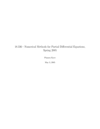
Consider the numerical solution to ut + aux = 0 with initial data u(0, x) = eiξ0 x p(x), where p(x) decays
rapidly at ∞. The function u(0, x) is called a wave packet—see Figure 1.1.
1
0.8
0.6
0.4
0.2
0
−0.2
−0.4
−0.6
−0.8
−1
−1 −0.5 0 0.5 1 1.5 2
πx
Figure 1.1: Wave packet cos 5π cos2 2 on [−1, 1]
The exact solution is u(t, x) = eiξ0 (x−at) p(x − at).
Proposition 1. A finite difference scheme will have a solution that is approximately
v ∗ (t, x) = eiξ0 (x−α(hξ0 )t) p(x − γ(hξ0 )t),
where α(hξ0 ) is the phase speed, and γ(hξ0 ) is the group velocity, given by
γ(θ) = α(θ) + θα (θ).
The rest of this section is devoted to proving Proposition 1 and may be skipped on a first reading.
Consider a class of one-step schemes with the property
v n (ξ) = g(hξ)ˆn−1 (ξ) = . . . = (g(hξ))n v 0 (ξ).
ˆ v ˆ
In addition, for simplicity, assume |g(hξ)| = 1. The numerical method will give
π/h
n 1
vm = √ eiξxm (g(hξ))n v 0 (ξ)dξ.
ˆ
2π −π/h
On the other side ∞
1
u(0, mh) = √ eimhξ u(0, ξ)dξ.
ˆ
2π −∞
∞ 2π
Split up the interval (−∞, ∞) = l=−∞ [l h − π , l 2π + π ) to obtain
h h h
l 2π + π
1 h h
u(0, mh) = √ eimhξ u(0, ξ)dξ.
ˆ
2π l l 2π − π
h h
Set ξ = l 2π
h + ξ , meaning dξ = dξ and
π
1 h 2π 2π
u(0, mh) = √ eimh(l h +ξ )
u(0, l
ˆ + ξ )dξ
2π −π h
l h
π ∞
1 h 2π
= √ eimhξ u(0, ξ + l
ˆ )dξ .
2π −π h
h l=−∞
16. 16 CHAPTER 1. HYPERBOLIC PDES
This gives a formula for
∞
2π
v 0 (ξ) =
ˆ u(0, ξ + l
ˆ ).
h
l=−∞
If u is smooth, then its Fourier transform decays rapidly, and only the middle l = 0 term really matters
v 0 (ξ) ∼ u(0, ξ),
ˆ ˆ
with the error bounded by h to some high power depending on the smoothness of u(0, x).
Consider
∞
1
u(0, ξ) =
ˆ √ e−ixξ u(0, x)dx
2π −∞
∞
1
= √ e−ixξ eiξ0 x p(x)dx
2π −∞
∞
1
= √ e−ix(ξ−ξ0 ) p(x)dx
2π −∞
= p(ξ − ξ0 )
ˆ
Let’s recall how we handle the phase speed
−i ωnk ξ ω
g(hξ) = |g(hξ)|e−iω = e−iω ⇒ (g(hξ))n = e−iωn = e = e−i λhξ tξ = e−iα(hξ)tξ .
k hξ
n
We can return to
π/h
1
n
vm = √ eiξxm · e−iα(hξ)tn ξ · v 0 (ξ)dξ.
ˆ
2π −π/h
2π
Exercise 1. Verify that eiξxm , v 0 (ξ), g(hξ), and ω are periodic functions of ξ with period
ˆ h .
Since v 0 (ξ) ∼ u(0, ξ) = p(ξ − ξ0 ), we change the variables φ = ξ − ξ0 . Then ξ = φ + ξ0 , and
ˆ ˆ ˆ
π/h+ξ0
1
n
vm = √ ei(φ+ξ0 )xm · e−iα(h(φ+ξ0 ))tn (φ+ξ0 ) · v 0 (φ + ξ0 )dφ.
ˆ
2π −π/h+ξ0
2π
Since all functions are periodic with period h we can shift the interval of integration back and get
π/h
1
n
vm = √ ei(φ+ξ0 )xm · e−iα(h(φ+ξ0 ))tn (φ+ξ0 ) · v 0 (φ + ξ0 )dφ.
ˆ
2π −π/h
This begins to look right. Factor out the phase speed
π/h
1
vm = eiξ0 (xm −α(hξ0 )tn ) · √
n
eiφxm · e−i[(φ+ξ0 )α(hφ+hξ0 )−ξ0 α(hξ0 )]tn · v 0 (φ + ξ0 )dφ.
ˆ
2π −π/h
This begins to look like a Fourier transform
π/h
1
“ ”
(φ+ξ0 )α(hφ+hξ0 )−ξ0 α(hξ0 )
iφ x− t
∼ eiξ0 (x−α(hξ0 )t) · √ e φ
· v 0 (φ + ξ0 )dφ.
ˆ
2π −π/h
Since v 0 (ξ) ∼ p(ξ − ξ0 ) we have v 0 (φ + ξ0 ) ∼ p(φ + ξ0 − ξ0 ) = p(φ). The next step is to replace v 0 (φ + ξ)
ˆ ˆ ˆ ˆ ˆ ˆ
by p(φ). Also since p(φ) goes to zero rapidly as φ → ∞ we may as well let the integral go to infinity. Hence
ˆ ˆ
∞
1
vm ∼ eiξ0 (x−α(hξ0 )t) · √
n
eiφ(x−˜ t) · p(φ)dφ = eiξ0 (x−α(hξ0 )t) · p(x − γ t).
γ
ˆ ˜
2π −∞
17. 1.7. GROUP VELOCITY AND PROPAGATION OF WAVE PACKETS 17
The last step is wrong because γ depends on φ, but it does tell us where we are going. We have
˜
(φ + ξ0 )α(hφ + hξ0 ) − ξ0 α(hξ0 )
γ
˜ ≡
φ
(hφ + ξ0 )α(hφ + hξ0 ) − hξ0 α(hξ0 )
=
hφ
(θ + θ0 )α(θ + θ0 ) − θ0 α(θ0 )
=
θ
G(θ + θ0 ) − G(θ0 )
=
θ
= G (θ0 ) + θ G (θ∗ ),
2
where θ ≡ hφ, θ0 ≡ hξ0 and G(θ) ≡ θα(θ) and θ∗ is between θ0 and θ. The beauty of the above expression
is that G (θ0 ) does not depend on φ, but only on hξ0 = θ0 .
Let’s go back to
π/h
1 hφ
(θ ∗ )t
vm ∼ eiξ0 (xm −α(hξ0 )tn ) · √
n
eiφ(xm −G (hξ0 ))tn · e−iφ 2 G p(φ)dφ.
ˆ
2π −π/h
hφ
(θ ∗ )t
The idea is to replace e−iφ 2 G by one. By doing so we are making an error bounded by
∞
hφ
(θ ∗ )t
e−iφ 2 G − 1 · |ˆ(φ)|dφ.
p
−∞
We will now show that this error is at most O(h).
Let’s first bound |ˆ(φ)|
p
∞
1
p(φ)
ˆ = √ e−iφx p(x)dx
2π −∞
∞
1
φ4 p(φ)
ˆ = √ (−iφ)4 e−iφx p(x)dx;
2π −∞
∞
1 ∂ 4 −iφx
= √ (e ) · p(x)dx
2π −∞ ∂x4
∞
1
= √ e−iφx · p (x)dx
2π −∞
Thus ∞
1 |p (x)|dx C
|ˆ(φ)| ≤ √ · −∞
p 4
= .
2π |φ| |φ|4
Also |eiz − 1|2 = 4 sin2 z
2 ≤ |z|2 , so |eiz − 1| ≤ |z|. By using this estimate we have
∞ ∞
hφ
(θ ∗ )t 1
e−iφ 2 G − 1 · |ˆ(φ)|dφ
p ≤ hφ2 G (θ∗ )t · |ˆ(φ)|dφ
p
−∞ −∞ 2
∞
≤ h · const · |φ2 p(φ)|dφ
ˆ
−∞
∞
1
≤ h · const · dφ
−∞ φ2
≤ h · const.
If we work in L2 we can bound the error by h2 in norm, but not pointwise.
Either way we have shown that
vm = eiξ0 (x−α(hξ0 )t) p(x − G (hξ)t) + small terms.
n
18. 18 CHAPTER 1. HYPERBOLIC PDES
Definition 9. The quantity γ(θ) = G (θ) = α(θ) + θ · α (θ) is called group velocity.
We have α(θ) → a as h → 0. So the phase speed is different from the group velocity, but both tend to
the correct speed a as h → 0. Otherwise the numerical method will not converge.
1.8 Summary of Schemes for the Wave Equation ut + aux = 0
k
Notation: λ = h , θ = hξ.
Name Scheme g(θ) Stable dissipative α(θ)/a
n+1 n n n
vm+1 −vm
Forward time vm −vm
k +a h =0
forward space
n+1 n n n
vm −vm−1
Forward time vm −vm order 2, if
k +a h = 0 1 − aλ + aλe−iθ 0 ≤ aλ ≤ 1
backward space 0 < aλ < 1
n+1 n n n
vm+1 −vm−1
Forward-time vm −vm
k + a 2h =0 1 − iaλ sin θ No No
centered space
Backward-time n n−1 vn −v n
vm −vm θ2
k + a m+12h m−1 =0 1− 6 (1 + 2a2 λ2 )
centered space
n+1 n aλ n n
vm =vm − 2 (vm+1 − vm−1 ) 1 − 2a2 λ2 sin2 θ
1 2
Lax–Wendroff a 2 λ2 n n n
2 |aλ| ≤ 1 order 4 1− 6 θ (1 − a2 λ2 )
+ (vm+1 − 2vm + vm−1 ) −iaλ sin θ
2
n+1 n
vm − 1 (vm+1 +vm−1 )n
2 2
Lax–Friedrichs mn
k
−v n
cos θ − iaλ sin θ |aλ| ≤ 1 No 1 + (1 − a2 λ2 ) θ3
+a m+1 m−1 = 0
2h
atan √ aλ sin θ
n+1
vm −vm n−1 vn −v n −iaλ sin θ 1−(aλ sin θ)2
Leap-Frog + a m+12h m−1 =0 p |aλ| < 1 No
2k ± 1 − (aλ sin θ)2 a
n+1
vm −vm n
k + 1− 1 iaλ sin θ θ2 1 2 2
Crank–Nicolson 2 Always No 1− (1 +
v
n+1
−v
n+1
+v n −v n 1+ 1 iaλ sin θ 6 2a λ )
a m+1 m−14h m+1 m−1 =0 2
19. Chapter 2
Parabolic equations
2.1 The Heat Equation
ut = buxx
Schemes:
• Lax–Friedrichs
vm − 1 (vm+1 + vm−1 )
n+1 n n
v n − 2vm + vm−1
n n
2
= b m+1 2
k h
• Lax–Wendroff
k2
u(t + k) = u + kut + utt
2
k 2 b2
= u + kbuxx + uxxxx
2
v n − 2vm + vm−1
n n n n n n n
k 2 b2 vm+2 − 4vm+1 + 6vm − 4vm−1 + vm−2
n+1
vm = vm + kb m+1
n
+ ·
h2 2 h4
• Forward in time, centered in space
n+1 n
vm − vm n n
v n − 2vm + vm−1
= b m+1
k h2
• Backward in time, centered in space
n+1 n
vm − vm v n+1 − 2vm + vm−1
n+1 n+1
= b m+1
k h2
• Leap-Frog
n+1
vm − vm n−1 v n − 2vm + vm−1
n n
= b m+1
2k h2
• Du Fort–Frankel
n+1
vm − vm n−1 v n − (vm + vm ) + vm−1
n+1 n−1 n
= b m+1
2k h2
• Crank–Nicolson
n+1 n+1 n+1
n+1 n
vm − vm b vm+1 − 2vm + vm−1 v n − 2vm + vm−1
n n
= + m+1 .
k 2 h2 h2
19
20. 20 CHAPTER 2. PARABOLIC EQUATIONS
For parabolic equations it appears natural to have a “new” λ, which we will call µ.
Definition 10 (µ).
k
µ≡ .
h2
Von Neumann analysis works the same way: vm = g n eimhξ .
n
Example 6. Forward in time, centered in space.
hξ
g(hξ) = 1 − 4bµ sin2 2 .
Stability requires |g| ≤ 1, i.e.,
hξ
0 ≤ 4bµ sin2 2 ≤2 for all |hξ| ≤ π, meaning bµ ≤ 1 .
2
The scheme is dissipative of order 2 as long as bµ is strictly less than 1 (check!). For bµ = 1 we have
2 2
g = 1 − 2 sin2 hξ and the frequency ξ = π is not damped at all: vm = eimhξ = eimπ = (−1)m remains
2 h
0
unchanged by the scheme.
Definition 11. Let
1
∞ 2
2
u(t, x) x ≡ |u(t, x)| dx
−∞
mean the L2 norm of u(t, x) with respect to x for a fixed t.
2
Remark 2. Let u be a solution to ut = buxx . Then the overall energy E(t) ≡ u(t, x) x decreases with time
u(t, x) x ≤ u(s, x) x, when t ≥ s
and the solution becomes smoother with time
2 1
ux (t, x) x ≤ u(0, x) 2 .
2bt
The dissipative schemes possess the same qualities
v n+1 = v n+1 = g(hξ)ˆn ≤ v n = v n
ˆ v ˆ
and
4µ 0 2
δ+ v n 2
≤ v ,
Ct
vm+1 −vm
where δ+ vm ≡ h , and C is a constant.
Proof. We will show that E (t) ≤ 0 meaning E(t) is decreasing:
∞ ∞ ∞ ∞
E (t) = 2uut dx = 2buuxx dx = 2buux − 2b u2 dx = −2b ux
x
2
x ≤ 0,
−∞ −∞ −∞ −∞
because u(t, x) → 0 as x → ±∞ for u(t, x) x to exist.
The above implies (after integrating from 0 to t):
t t
2 2
E(t) − E(0) = −2b ux (τ, x) x dτ ⇒ E(0) ≥ 2b ux (τ, x) x dτ
0 0
∂
The derivative ux = ∂x u(t, x) is also a solution to ut = buxx because (ux )t = (ut )x = buxxx = b(ux )xx ,
therefore ux (t, x) x ≤ ux (s, x) x for t ≥ s. Now we get
t
2 2
E(0) ≥ 2b ux (τ, x) x dτ ≥ 2bt ux (t, x) x,
0
21. 2.1. THE HEAT EQUATION 21
meaning
1 2
ux (t, x) u(0, x) 2 ,
xx ≤
2bt
i.e., the solution get smoother and smoother as t → ∞.
Now repeat the same analysis for a difference scheme that is dissipative of order (say) 2:
hξ
v n+1 (ξ) = g(hξ)ˆn (ξ),
ˆ v where |g(hξ)| ≤ 1 − C sin2 2 ,
which implies
2
hξ
v n+1 (ξ)
ˆ 2
≤ 1 − C sin2 2 v n (ξ)
ˆ
and (after some major reworking):
2
v n+1
ˆ 2
+ C sin hξ · v n
2 ˆ ≤ vn
ˆ 2
(these are, of course, the discrete L2 norms). Now comes the big moment,
eihξ/2 − e−ihξ/2 n e−ihξ/2 ihξ
sin(hξ/2) · v n (ξ) =
ˆ · v (ξ) =
ˆ (e − 1)ˆn (ξ).
v
2i 2i
Next, observe that
π/h
n 1 n n 1 eihξ − 1 n
δ+ vm ≡ (v − vm ) = √ eimhξ v (ξ)dξ.
ˆ
h m+1 2π −π/h h
On the other side,
π/h
n 1
δ+ vm = √ eimhξ δ+ v n (ξ)dξ,
2π −π/h
so
eihξ − 1 n
v (ξ) = δ+ v n (ξ),
ˆ
h
and inserting we get
sin(hξ/2) · v n =
ˆ 1
2 (eihξ − 1)ˆn =
v 1
2 · h · δ+ v n .
We can therefore simplify our inequality
h2
v n+1
ˆ 2
+C δ+ v n 2
≤ vn 2 .
ˆ
4
Parseval says “hats = no hats”, so
Ck
v n+1 2
+ δ+ v n 2
≤ vn 2 , (2.1)
4µ
where, again, µ = k/h2 . In particular,
v n+1 ≤ v n .
Next, we prove that δ+ v n+1 ≤ δ+ v n . The only property we used was that vm was solution to
n
n+1 n
vm − vm v n − 2vm + vm−1
n n
= b m+1 .
k h2
Now try
n+1 n
vm+1 − vm+1 v n − 2vm+1 + vm
n n
= b m+2 .
k h2
22. 22 CHAPTER 2. PARABOLIC EQUATIONS
Subtract first from second, divide by h and get
n+1 n+1 n n n n n n n n
vm+1 −vm vm+1 −vm vm+2 −vm+1 vm+1 −vm vm −vm−1
h − h h −2 h + h
=b .
k h2
Or in a simpler language
(δ+ v)n+1 − (δ+ v n )m
m (δ+ v)n n n
m+1 − 2(δ+ v)m + (δ+ v)m−1
=b ,
k h2
meaning δ+ v n+1 ≤ δ+ v n .
The inequality (2.1) works for all time steps
Ck
v n+1 2
+δ+ v n 2
≤ vn 2
4µ
Ck
vn 2
+ δ+ v n−1 2
≤ v n−1 2
4µ
.
.
.
Ck
v1 2
+ δ+ v 0 2
≤ v0 2 ,
4µ
which we sum up and cancel common terms to obtain
n
Ck
v n+1 2
+ δ+ v k 2
≤ v0 2
⇒
4µ
k=0
Ck(n + 1)
v n+1 2
+ δ+ v n+1 2
≤ v0 2
⇒
4µ
4µ 0 2
δ+ v n+1 2
≤ v .
Ct
This means that the numerical solution will smooth out—as long as the scheme is dissipative.
23. 2.2. THE DU FORT–FRANKEL SCHEME 23
2.2 The Du Fort–Frankel Scheme
This is an example of an explicit and unconditionally stable scheme for ut = buxx .
The problem with schemes like forward time, centered space is that they are stable for bµ = bk/h2 ≤ 1 ,
2
2
which puts a terrible restriction k ≤ h on the timestep. The Du Fort–Frankel scheme,
2b
n+1 n−1 n n+1 n−1 n
vm − vm = 2bµ(vm+1 − (vm + vm ) + vm−1 ),
is a slight modification of the unstable Leap–Frog scheme. We rewrite the Du Fort–Frankel scheme as
n+1 n−1 n n
(1 + 2bµ)vm − (1 − 2bµ)vm = 2bµ(vm+1 + vm−1 ).
To study the stability, we substitute vm = g n eimhξ to get
n
(1 + 2bµ)g 2 − (1 − 2bµ) = 2bµ(eihξ + e−ihξ )g,
which implies
2bµ cos(hξ) ± 1 − 4b2 µ2 sin2 (hξ)
g± = .
1 + 2bµ
The scheme is not dissipative since g− (π) = −1. To determine stability we consider two cases:
√
2bµ| cos(hξ)|+ 1 2bµ+1
• 1 − 4b2 µ2 ≥ 0 ⇒ |g± | ≤ 1+2bµ ≤ 1+2bµ = 1.
(2bµ cos(hξ))2 +4b2 µ2 cos2 (hξ)−1 4b2 µ2 −1 2bµ−1
• 1 − 4b2 µ2 < 0 ⇒ |g± |2 = 1+2bµ = (1+2bµ)2 = 1+2bµ ≤ 1.
In addition, we do not want double roots on the unit circle. Double root occurs when 1 − 4b2 µ2 = 0, but
then |g± | ≤ 2bµ| cos(hξ)| < 1.
1+2bµ
So we have stability for any value of µ. But how is that possible? The catch is in the consistency. In
order for the scheme to be consistent we must have k/h → 0, as we will now demonstrate.
Rewrite Du Fort–Frankel as
n+1
vm − vm n−1 v n − 2vm + vm−1
n n
v n+1 + vm − 2vm
n−1 n
= b m+1 −b m
2k h2 h2
then expand in Taylor to see that it approximates
k2 h2 k2 k4
ut + uttt = b uxx + uxxxx − b 2 utt + utttt .
6 12 h 12h2
k
Now think numerically. For hyperbolic systems we could (at best) hope for h ≈ 1. However, if we use Du
Fort–Frankel with such a timestep, k = h, the solution will not converge to the solution of ut = buxx , but
instead to the solution of butt + ut = buxx (i.e., the solution to a wave equation). This was not the purpose of
k
the exercise. So the scheme will only converge to the solution of ut = buxx if h → 0. Even so the truncation
k2 k
error will be dominated by b h2 utt , which is not small unless h2 is constant, but then we are back where we
started—with the same restrictions as the ones for forward in time centered in space.
We, of course have two explicit schemes—backward in time, centered in space (which is O(k + h2 ) and
k
dissipative) and Crank–Nicolson (which is O(k 2 + h2 ) and not dissipative if h is constant.).