
Empfohlen
Empfohlen
Weitere ähnliche Inhalte
Was ist angesagt?
Was ist angesagt? (19)
Andere mochten auch
Ähnlich wie Patriarca_3668.ppt
Ähnlich wie Patriarca_3668.ppt (20)
Mehr von grssieee
Mehr von grssieee (20)
Kürzlich hochgeladen
Kürzlich hochgeladen (20)
Patriarca_3668.ppt
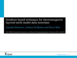
- 1. Gradient based technique for electromagnetic layered earth model data inversion Claudio Patriarca, Andrea Di Matteo and Evert Slob 2011 IEEE Internation Geoscience and Remote Sensing Symposium, Vancouver BC, July 2011
- 2. Local or Global inversion Inversion Schemes Gradient descent Global Multilevel Coordinate search
- 4. Towards local inversion Objective Function Jacobian Jacobian calculation †
- 6. Local Full-waveform inversion Numerical test case #1: smooth model
- 7. Local Full-waveform inversion Numerical test case #1 result h 2 (m) ε q · 10 -3 m ε m ϕ Model Parameters 0,10 35 4,5 - GMCS 0,10 24 3.0 0,135 Gradient 0,10 17 3,7 0,135
- 9. Local Full-waveform inversion Real data test case
- 10. Local Full-waveform inversion Real data test case results h 1 (m) h 2 (m) ε 2 log σ 2 (Sm -1 ) ϕ GMCS 0,19 0,15 6,08 -1,06 0,24 Gradient 0,19 0,14 5,51 -1,01 0,25
- 11. Local Full-waveform inversion Numerical test case #2: piecewise layered half-space
- 12. Objective Function topography Numerical test case #2: piecewise layered half-space Global Minimum ε 1 ε 2 h 2
Hinweis der Redaktion
- Let me briefly summarize the main differences between local and global inversion algorithms. The axes in these pictures represent one parameter pair, and the curves represent objective function values. Local inversion methods are sensitive to gradients in the mismatch and move effectively downhill, but generally become trapped in local minima and must be initiated from a large number of starting points. Global inversion methods use a directed more or less random process to search the parameter space for the optimal solution. They include the ability to escape from local minima, but as no gradient information is used, the search can be relatively inefficient
- EM inversion is a nonlinear geophysical inverse problem for which a direct solution is not available. These problems can be formulated by assuming a discrete form of the model by assigning different parameters to the vector valued parameter b that is used to generate a modeled Green’s function; this modeled Green’s function is used in the objective or cost function phi( b ) which represents the mismatch between the measured data and replica data computed for a particular model configuration This can be a challenging problem due to: the size of the parameter space, which increases geometrically with the number of parameters; the presence of many local minima due to the nonlinearity of the inverse problem; correlations between parameters that pose a limit to parameter sensitivity. This problem is intractable using global inefficient techniques Gradient methods: trust region reflective and Levenberg-Marquardt
- Therefore we decide to move to local inversion algorithms. The normalization with respect to the measured Green’s function can be treated as a multiplication of the multiparameter objective function for a frequency independent constant function alpha , such that the minimization problem can be written as… therefore objective function partial derivatives reduce to the modeled Green’s function partial derivative with respect to the same parameter (bn), and the gradient problem is then reduced to the jacobian of the modelled green’s function [The best linear approximation of the multivariate es timated function G xx (b , ω ) is represented by its Jacobian in any given point within the search space. The matrix of the partial derivatives with respect to model parameters can be expressed for every particular model configuration]
- The adavantage in using the explicit gradient of the objective function is clearly visible when a relatively easy monotone complex function gradient is numerically evaluated. The function y is plot for a certain range of values, to which random noise is added to mimic real data. Despite the numerically evaluated jacobian respect to parameters a and b is not accurate, the estimated function y is still well retrieved. However, it is desirable to have correct jacobian to avoid computational instability and to be able to retrieve the correct function will less uncertainty and more accuracy.
- This testcase involved determining the EM and geometric properties for the environment shown in the picture. In this testcase, the form of the EM model is known to consist of a single layer over a perfect electric conductor. There are X unknown parameters including the source height, h0, layer thickness, constant electric conductivity and electric permittivity – linear gradient assumed. The true parameter values and the assumed lower and upper parameter bounds are given in the picture. A smooth model can be implemented, where the function G xx (b , ω ) and the reflection coefficients depend on smoothly varying model parameters. In the forward model the constitutive parameter εn linearly changes with depth d . The electric permittivity is only considered to vary inside the layer of interest, and a simple linear relationship is adopted, so that ε n = ε q + ε m ・ Δ d, where εq represents the electric permittivity starting values at the top of the interface, and εm accounts for the linear increase of permittivity with depth d . This model can be particularly useful, for example, in case of internal zonation in concrete or for investigations in the vadose zone where permittivity tends to smoothly increase with depth. The data consist of a numerical Green’s function measured in monostatic mode over a ultra wide BW ranging from 3 to 8 GHz. The measure of mismatch adopted in this study is based on the normalized objective function summed over multiple frequency values.
- A great advantage is offered by the local inversion schemes in terms of computational time. When a dense grid of measurements in set, as it is the case for non-destructive testing applications, inefficient inversion schemes cannot be tolerated to quantitatively invert for big datasets. The picture shows a monostatic horn antenna acquisition during a field campaign in the theater of Megalopolis in Greece, where EM characterization of the entire element in the picture was to be carried out.
- Inversion for the model parameters are performed in a relatively large param eter space . Despite the curve fit of both inversion schemes are comparable in both frequency and time domain, a considerable advantage in inversion time is again given by the gradient method that reaches convergence faster, up to three orders of magnitude compared to GMCS.
- The presence of local minima is visually investigated for the relatively simple model configuration shown in the picture: a single layer above an halfspace of given permittivity and conductivity. The movies shows the changes on the objective function (change in colour) for given values of relative permittivity (in abscissa and ordinate axes), in the direction of depth within layer 2.
- Local inversion methods are sensitive to local gradients in the mismatch and move effectively downhill, but typically become trapped in local minima. Optimum gradient and on global search were compared in performing numerical and real data inversions. the gradient technique resulted in a cheap computation method usable in specialized applica tions (multilayering, large datasets) that are intractable with global optimization techniques. in the implemented smooth model, where the function G xx (b , ω ) and the reflection coefficients depend on smoothly varying model parameters, the gradient technique performs as well as the global minimization, with a considerable advantage in time inversion. The same advantage is observed in real data inversion. The capability of deep interfaces inversion will be investigated, because it is known that the inversion resolution and signal-to-noise ratio decreases with depth. Second order derivatives can be calculated to compute the inverse of the Hessian, which allows to follow the curvature and further improve the convergence, but the implementation of the Hessian may not be cost-efficient. (Limited precision numerical data additive and multiplicative noise that mimic real data can be used to obtain estimates of the accuracy of inverted values)