R tool

1. Introduction to R
1. Before installing Studio your system must have R in your system.
a. First install R and then try to install Rstudio
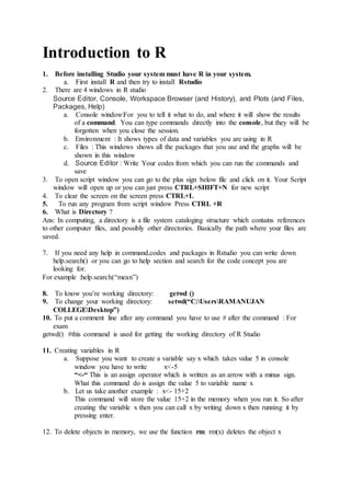
2. There are 4 windows in R studio
Source Editor, Console, Workspace Browser (and History), and Plots (and Files,
Packages, Help)
a. Console window:For you to tell it what to do, and where it will show the results
of a command. You can type commands directly into the console, but they will be
forgotten when you close the session.
b. Environment : It shows types of data and variables you are using in R
c. Files : This windows shows all the packages that you use and the graphs will be
shown in this window
d. Source Editor : Write Your codes from which you can run the commands and
save
3. To open script window you can go to the plus sign below file and click on it. Your Script
window will open up or you can just press CTRL+SHIFT+N for new script
4. To clear the screen on the screen press CTRL+L
5. To run any program from script window Press CTRL +R
6. What is Directory ?
Ans: In computing, a directory is a file system cataloging structure which contains references
to other computer files, and possibly other directories. Basically the path where your files are
saved.
7. If you need any help in command,codes and packages in Rstudio you can write down
help.search() or you can go to help section and search for the code concept you are
looking for.
For example :help.search(“mean”)
8. To know you’re working directory: getwd ()
9. To change your working directory: setwd(“C:UsersRAMANUJAN
COLLEGEDesktop”)
10. To put a comment line after any command you have to use # after the command : For
exam
getwd() #this command is used for getting the working directory of R Studio
11. Creating variables in R
a. Suppose you want to create a variable say x which takes value 5 in console
window you have to write x<-5
“<-“ This is an assign operator which is written as an arrow with a minus sign.
What this command do is assign the value 5 to variable name x
b. Let us take another example : x<- 15+2
This command will store the value 15+2 in the memory when you run it. So after
creating the variable x then you can call x by writing down x then running it by
pressing enter.
12. To delete objects in memory, we use the function rm: rm(x) deletes the object x

2. 13. You can simply type an expression without assigning its value to an object, the result is
thus displayed on the screen but is not stored in memory. For example: (10+5)*4 or
sqrt(16)
14. If you run a command which is incomplete say
>Sqrt(16
R studio will show an error : Error: unexpected symbol in:
"sqrt(14
sqrt"
15. To generate sequence of say 1 to 100 and save it as variable x. Colons here represent
“to”.
>x<-1:100
16. To generate sequence of say 1 to 100 and save it as variable x. Colons here represent
“to”.
>x<-1:100
17. If you want save a variable y with a sequence with a gap of 2 within range 1 to 100
>y<-seq(1,100,2)
18. If you want to repeat 3 six times.
>rep(5,6)

3. 19. If you want to create an vector say x which can take more than one values say 8,9,10,15.
>x=c(8,9,10,15) # c is function used to combine two or more values it is called
concatenate function “c”
20. Suppose you want to add two vectors x and y with values (8,9,10,15) and (1,2,3,4)
respectively and then store the added value (x+y) value in z.
>x<-c(8,9,10,15)
>y=c(1,2,3,4)
> z =x+y
21. Suppose you want first create a data of 5 students age in certain class with age 5,6,7,8
and 9. Then want to find there average age, median age, standard deviation, min, max
and range.
>age<-c(5,6,7,8,9)
>mean(x) # mean() is used to calculate mean or average of any variable.
>median(age) # median() is used to calculate median
>sd(age) # sd() is used for standard deviation
>min(age) #min() is used minimum
>max(age) #max() is used for maximum
>range(age) #range of variable (5-9)
22. If you use summary command it will give you summary of the variable which includes
minimum, 1 quartile,median,meand,3rd quartile, maximum.
>summary(age)
23. If you want to add any character or string values in your variable. Suppose I want to
create a variable x with the names of 5 students in your class ravi,vipin,ashish,sahil,sachin
.
>y<-c(“ravi”,”vipin”,”ashish”,”sahil”,”sachin”) # so if you are using any string or
character you must use “charater” for input in R.

4. 24. If you want to create a matrix Matrix. A matrix is actually a vector with an additional
attribute (dim) which is itself a numeric vector with length 2, and defines the numbers of
rows and columns of the matrix. A matrix can be created with the function matrix().
Default function is: matrix(data = NA, nrow = 1, ncol = 1, byrow = FALSE,
dimnames = NULL). nrow represents the number of row and ncol represents number of
columns.
The option byrow indicates whether the values given by data must fill successively the
columns (the default) or the rows (if TRUE). The option dimnames allows to give names
to the rows and columns.
For example:
>x<-matrix(c(1,2,3,4,5,6,7,8,9),nrow=3,ncol=3,byrow=T) # matrix would be in row
form
>y<-matrix(c(1,2,3,4,5,6,7,8,9),nrow=3,ncol=3,byrow=T) # matrix would be in column
form
25. If you want to add ,multiply two A and B matrix
>A<-matrix(c(1,2,3,4,5,6,7,8,9,),nrow=3,ncol=3,byrow=T) # matrix would be in row
form
>B<-matrix(c(10,20,30,40,50,60,70,80,90),nrow=3,ncol=3,byrow=T) # matrix would be
in row form
>A+B
>A%*%B

5. 26. If you want transpose and determinant of matrix A
>t(A) # Transpose of matrix
>det(A) #Determinant of matrix
27. If you want sum of rows and sum of columns:
>rowSums(A) # it will add the values of the rows in an matrix
>ColSums(A) # it will add the values of the Columns in an matrix
28. If you eignenvalue and eigenvector of vectors.
>eigen(A) # for eigen vectors and eigen values

6. 29. If you want to create a data you can use data.frame()
>Patient_ID=c(1,2,3,4,5,6,7) # Creating a variable for patient ID
>age=c(25,34,28,52,44,47,78) # creating a variable for patient age
>diabeties=c(“t1”,”t1”,t2”,”t1”,”t1”,”t2”,”t2”) # Creating a variable if the patient is Type
1 or Type 2
>sugar_level=c(180,162,120,145,180,137,102) # creating a variable of sugar level of
patient
>dat=data.frame(Patient_ID,age,diabeties,sugar_level) # creating data with variable
name dat
>dat # calling the data

7. 30. If you want to import excel file(.csv format file) in R :
a. >Data=read.csv(file.choose(),header=T) and clicking on the file
Header means a logical value indicating whether the file contains the names of the
variables as its first line. If missing, the value is determined from the file format: header is
set to TRUE if and only if the first row contains one fewer field than the number of
columns
b. >Data=read.csv(file.choose(“C:UsersRAMANUJAN COLLEGEDesktop”),header=T)
#reading .csv file
31. If you want to see first six observation of data
>head(data)
32. If you want to see last six observation of data
>tail(data)
33. If you want to import data which is in text form:
>dat=read.table(“C:UsersRAMANUJAN COLLEGEDesktop”)
34. If you want to call a specific variable say age in some data file saved in your Rstudio as
“data”.
>dat$age # “$” sign is used to call a specific variable after the file name
35. Summary of specific variable in your data set
>summary(dat$age)
36. If you want to save the data file :
write.csv(Your DataFrame,"Path where you'd like to export the DataFrameFile Name.csv",
row.names = FALSE)

8. Plotting graphs in R
1. A bar chart represents data in rectangular bars with length of the bar proportional
to the value of the variable. R uses the function barplot() to create bar charts. R
can draw both vertical and Horizontal bars in the bar chart. In bar chart each of
the bars can be given different colors.
>barplot(mydata,beside,xlab,ylab,main,col)
Following is the description of the parameters used −
 mydata :Data you want to enter
 beside :a logical value. If FALSE, the columns of height are portrayed as
stacked bars, and if TRUE the columns are portrayed as juxtaposed bars.
 xlab is the label for x axis.
 ylab is the label for y axis.
 main is the title of the bar chart.
 col is used to give colors to the bars in the graph.
2. Pie chart is created using the pie() function which takes positive numbers as a
vector input.
Syntax
The basic syntax for creating a pie-chart using the R is −
pie(mydata,beside, labels, main, col, clockwise)
Following is the description of the parameters used −
 mydata is a vector containing the numeric values used in the pie chart.
 labels is used to give description to the slices.
 main indicates the title of the chart.
 col indicates the color palette.
 clockwise is a logical value indicating if the slices are drawn clockwise or
anti clockwise.
3. Histogram represents the frequencies of values of a variable bucketed into
ranges.
R creates histogram using hist() function. This function takes a vector as an input
and uses some more parameters to plot histograms.
Syntax
The basic syntax for creating a histogram using R is −

9. hist(mydata,main,xlab,xlim,ylim,density,breaks,col)
Following is the description of the parameters used −
mydata is a vector containing numeric values used in histogram.
main indicates title of the chart.
col is used to set color of the bars..
density: how the data is dense
xlab is used to give description of x-axis.
xlim is used to specify the range of values on the x-axis.
ylim is used to specify the range of values on the y-axis.
breaks is used to mention the width of each bar.
4. Boxplots are a measure of how well distributed is the data in a data set. It divides
the data set into three quartiles.
Boxplots are created in R by using the boxplot() function.
Syntax
The basic syntax to create a boxplot in R is −
boxplot(Mydata,names, main,xlab,ylab,col)
Following is the description of the parameters used −
Mydata is a vector or a formula.
names are the group labels which will be printed under each boxplot.
main is used to give a title to the graph.
Xlabis used to give description of x-axis.
Ylabis used to give description of y-axis.
Col is for choosing color of the graph
5. Scatterplots show many points plotted in the Cartesian plane. Each point
represents the values of two variables.
The simple scatterplot is created using the plot() function.
Syntax
The basic syntax for creating scatterplot in R is −
plot(x, y, main, xlab, ylab, xlim, ylim, axes,col)
Following is the description of the parameters used −
 x is the data set whose values are the horizontal coordinates.
 y is the data set whose values are the vertical coordinates.

10.  main is the tile of the graph.
 xlab is the label in the horizontal axis.
 ylab is the label in the vertical axis.
 xlim is the limits of the values of x used for plotting.
 ylim is the limits of the values of y used for plotting..
 Col is the colour of the graph
After this you can draw a regressionlin using abline()
6. A line chart is a graph that connects a series of points by drawing line segments
between them. These points are ordered in one of their coordinate (usually the x-
coordinate) value. The plot() function in R is used to create the line graph.
Syntax
The basic syntax to create a line chart in R is −
plot(mydata,type,col,xlab,ylab)
Following is the description of the parameters used −
 Mydata is a vector containing the numeric values.
 type takes the value "p" to draw only the points, "l" to draw only the lines and
"o" to draw both points and lines.
 xlab is the label for x axis.