SlideShare ist ein Scribd-Unternehmen logo
1 von 45
Activity Analysis, Cost
Behavior, and Cost
Estimation
Chapter 6
McGraw-Hill/Irwin Copyright © 2014 McGraw-Hill Education.
All rights reserved. No reproduction or distribution without the
prior written consent of McGraw-Hill Education.
Presenter
Presentation Notes
Chapter 6: Activity Analysis, Cost Behavior, and Cost
Estimation
Learning Objective1
6-2
Presenter
Presentation Notes
Learning Objective 1. Explain the relationships between cost
estimation, cost behavior, and cost prediction.
Cost
prediction
Using knowledge
of cost behavior
to forecast
level of cost at
a particular
activity. Focus
is on the future.
Introduction
Cost
behavior
Relationship
between
cost and
activity.
Process of
determining
cost behavior,
often focuses
on historical
data.
Cost
estimation
6-3
Presenter
Presentation Notes
How does a managerial accountant determine the cost behavior
pattern for a particular cost item?
The determination of cost behavior, which is often called cost
estimation, can be accomplished in a number of ways.
One way is to analyze historical data concerning costs and
activity levels.
The relationship between cost and activity, called cost behavior,
is relevant to the management functions of planning, control,
and decision making.
In order to plan operations and prepare a budget, managers need
to predict the costs that will be incurred at different levels of
activity.
Knowledge of cost behavior will help the manager to make the
desired cost prediction.
A cost prediction is a forecast of cost at a particular level of
activity. (LO1)
Learning Objective 2
6-4
Presenter
Presentation Notes
Learning Objective 2. Define and describe the behavior of the
following types of costs: variable, step-variable, fixed, step-
fixed, semivariable (or mixed), and curvilinear.
Total Variable Cost Example
Your total Pay Per View bill is based on how many Pay Per
View
shows that you watch.
Number of Pay Per View shows
watched
To
ta
l P
ay
P
er
V
ie
w
B
ill
6-5
Presenter
Presentation Notes
A variable cost changes in total in direct proportion to a change
in the activity level (or cost driver).
For example, assume that you pay $4.95 for each Pay Per View
show that you watch.
The more shows that you watch, the higher your Pay Per View
bill will be.
The total cost of the Pay Per View bill increases in direct
proportion to the number of shows watched.
Your text book describes the raw materials that goes into
making donuts are also variable costs―the more donuts you
make the higher the cost of raw materials. (LO2)
Variable Cost Per Unit Example
The cost per Pay Per View show is constant. For example,
$4.95
per show.
Number of Pay Per View
shows watched
C
os
t p
er
P
ay
P
er
V
ie
w
sh
ow
6-6
Presenter
Presentation Notes
However, the variable cost per unit is constant as activity
changes. In our Pay Per view example, the cost per show
remains at $4.95. To summarize, as activity changes, total
variable cost increases in direct proportion to the change in
activity level, but the variable cost per unit remains constant.
(LO2).
Step-Variable Costs
Activity
C
os
t
Total cost remains
constant within a
narrow range of
activity.
6-7
Presenter
Presentation Notes
Some costs are nearly variable, but they increase in small steps
instead of continuously.
Such costs, called step-variable costs, usually include inputs
that are purchased and used in relatively small increments.
For a narrow range of activity, the total cost remains the same.
For example, the hourly rate for cashiers at a local grocery store
is a set amount.
During hours when there are few customers only three cashiers
are needed.
Therefore, at these low activity levels, the total cost for cashiers
is the same. (LO2)
Step-Variable Costs
Activity
C
os
t
Total cost increases to a
new higher cost for the
next higher range of
activity.
6-8
Presenter
Presentation Notes
But when the number of customers increases, the number of
cashiers required increases.
The hourly rate, or cost per unit, stays the same but the total
cost increases at the next higher range of activity. (LO2)
Total Fixed Cost Example
Your monthly basic cable TV bill probably does not change no
matter
how many hours you watch.
Number of hours watched
M
on
th
ly
B
as
ic
C
ab
le
B
ill
6-9
Presenter
Presentation Notes
A fixed cost remains unchanged in total as the activity level
varies.
Examples of fixed costs include facilities costs, which include
property taxes, depreciation on buildings and equipment, and
the salaries of maintenance personnel.
The total cost of fixed costs remains constant, regardless of the
level of activity. (LO2)
Fixed Cost Per Unit Example
The average cost per hour decreases as more hours are spent
watching cable television.
Number of hours watched
M
on
th
ly
B
as
ic
c
ab
le
B
ill
pe
r
ho
ur
w
at
ch
ed
6-10
Presenter
Presentation Notes
However, the fixed cost per unit does change as activity varies.
The fixed cost per unit is calculated by dividing the total fixed
costs by the number of units. Therefore, as the activity level
increases, total fixed costs does not change, but unit fixed cost
declines. For this reason, it is preferable in any cost analysis to
work with total fixed cost rather than fixed cost per unit. (LO2)
Step-Fixed Costs
Example: Office space is
available at a rental rate of
$30,000 per year in increments
of 1,000 square feet. As the
business grows more space is
rented, increasing the total
cost.
Continue
6-11
Presenter
Presentation Notes
Some costs remain fixed over a wide range of activity but jump
to a different amount for activity levels outside that range.
Such costs are called step-fixed costs. (LO2)
R
en
t C
os
t i
n
Th
ou
sa
nd
s
of
D
ol
la
rs
0 1,000 2,000 3,000
Rented Area (Square Feet)
30
60
90
Total cost doesn’t change for a wide range of activity,
and then jumps to a new higher cost for the next
higher range of activity.
Step-Fixed Costs
6-12
Presenter
Presentation Notes
A company may rent office space at the cost of $30,000 per
1,000 square feet.
Extra space is only available in increments of 1,000 square feet.
The rent remains $30,000 regardless of activity.
As business increases, more square footage is needed.
The next 1,000 square feet costs another $30,000.
As the company expands, another 1,000 square feet is needed,
costing another $30,000. (LO2)
Step-variable costs
can be adjusted more
quickly and . . .
The width of the
activity steps is much
wider for the
step-fixed cost.
How does this type
of fixed cost differ
from a step-variable
cost?
Step-Fixed Costs
6-13
Presenter
Presentation Notes
Step-variable costs differ from step-fixed costs in that they can
be adjusted more quickly.
Also, the width of the steps is much wider for step-fixed costs.
(LO2)
Semivariable Cost
A semivariable cost
is partly fixed and
partly variable.
Consider the
following
example:.
6-14
Presenter
Presentation Notes
A semivariable (or mixed) cost has both a fixed and a variable
component.
Assume that a construction company leases a bulldozer and
incurs a flat fee of $1500 per month, regardless of how many
hours the bulldozer is used.
The company also incurs a cost of $35 per hour used. (LO2)
Fixed Monthly
Rental Charge
Variable Lease
Charge Per Hour
Rental Charge Per Hour
To
ta
l L
ea
se
C
os
t
Semivariable Cost
The slope is
the variable
cost per unit
of activity.
6-15
Presenter
Presentation Notes
The company’s monthly bill would always be at least $1,500,
the fixed portion of the lease.
The total cost would rise from $1,500, depending on how hours
were used.
Therefore, the slope of a total cost line is the variable cost per
unit of activity. (LO2)
Curvilinear Cost
Curvilinear
Cost Function
Relevant Range
Activity
To
ta
l C
os
t
Curvilinear
Cost Function
A straight-line
(constant unit
variable cost) closely
approximates a
curvilinear line within
the relevant range.
6-16
Presenter
Presentation Notes
The graphs of all of the cost behavior patterns examined so far
consist of either straight lines or several straight-line sections.
A curvilinear cost behavior pattern has a curved graph.
Assume that a company groups its trash collection, telephone
and electricity costs together as utility costs.
The company’s utilities cost may be a curvilinear cost. Recall
that a marginal cost is the cost of producing the next unit.
For low levels of activity, the utilities cost would exhibit
decreasing marginal costs because only the electricity costs
would increase as production increased.
For high levels of activity the graph would exhibit increasing
marginal costs.
If the demand for a particular month is at lower levels of
activity, the company can use its modern, energy efficient
equipment.
But at higher levels of activity, the older equipment must also
be used.
This equipment is less energy-efficient.
As a result, the marginal utilities cost rises as monthly activity
increases. (LO2)
Learning Objective 3
6-17
Presenter
Presentation Notes
Learning Objective 3. Explain the importance of the relevant
range in using a cost behavior pattern for cost prediction.
Curvilinear Cost
Curvilinear
Cost Function
Relevant Range
Activity
To
ta
l C
os
t
Curvilinear
Cost Function
A straight-Line
(constant unit
variable cost) closely
approximates a
curvilinear line within
the relevant range.
6-18
Presenter
Presentation Notes
Management need not concern itself with extreme levels of
activity if it is unlikely the company will operate at those
activity levels.
Management is interested in cost behavior within the company’s
relevant range, the range of activity within which management
expects the company to operate. (LO3)
Learning Objective 4
6-19
Presenter
Presentation Notes
Learning Objective 4. Define and give examples of engineered
costs, committed costs, and discretionary costs.
Engineered, Committed, and Discretionary
Costs
Discretionary
May be altered in the
short term by current
managerial decisions.
Committed
Long-term, cannot be
reduced in the short
term.
Engineered
Physical relationship
with activity measure.
Depreciation on
Buildings and
equipment
Advertising and
Research and
Development
Direct
Materials
6-20
Presenter
Presentation Notes
In the process of budgeting costs, it is often useful for
management to make a distinction between engineered,
committed, and discretionary costs.
An engineered cost bears a definitive physical relationship to
the activity measure. Direct-material cost is an engineered cost.
A committed cost results from an organization’s ownership or
use of facilities and its basic organization structure. Property
taxes, depreciation on buildings and equipment, costs of
renting facilities or equipment, and the salaries of management
personnel are examples of committed fixed costs.
A discretionary cost arises as a result of a management decision
to spend a particular amount of money for some purpose.
Examples of discretionary costs include amounts spent on
research and development, advertising and promotion,
management development programs, and contributions to
charitable organizations. (LO4)
Cost Behavior in Other Industries
Merchandisers
Cost of Goods Sold
Manufacturers
Direct Material, Direct
Labor, and Variable
Manufacturing Overhead
Merchandisers and
Manufacturers
Sales commissions and
shipping costs
Service Organizations
Supplies and travel
Examples of variable costs
6-21
Presenter
Presentation Notes
The cost behavior pattern appropriate for a particular cost item
depends on the organization and the activity base (or cost
driver). In manufacturing firms, production quantity, direct
labor hours, and machine hours are common cost drivers.
Direct-material and direct labor costs are usually considered
variable costs. Other variable costs include some
manufacturing-overhead costs, such as indirect material and
indirect labor. In merchandising firms, the activity base (or
cost driver) usually is sales revenue. The cost of merchandise
sold is a variable cost. Sales commissions and shipping costs
would be variable costs for both manufacturers and
merchandisers. In service organizations, supplies and travel
expenses are variable costs. (LO4)
Examples of fixed costs
Merchandisers, manufacturers, and
service organizations
Real estate taxes
Insurance
Sales salaries
Depreciation
Cost Behavior in Other Industries
6-22
Presenter
Presentation Notes
Property taxes, insurance expense, fixed salaries, depreciation
are all examples of fixed costs for manufacturers,
merchandisers, and service organizations. (LO4)
Learning Objective 5
6-23
Presenter
Presentation Notes
Learning Objective 5. Describe and use the following cost
estimation methods: account classification, visual fit, high-low,
and least-squares regression.
Account-Classification Method
Visual-Fit Method
High-Low Method
Least-Squares Regression Method
Cost Estimation
6-24
Presenter
Presentation Notes
Different costs exhibit a variety of cost behavior patterns.
Cost estimation is the process of determining how a particular
cost behaves.
Several methods are commonly used to estimate the relationship
between cost and activity.
Some of these methods are simple, while some are quite
sophisticated.
In some firms, managers use more than one method of cost
estimation.
The results of the different methods are then combined by the
cost analyst on the basis of experience and judgment. (LO5)
Account Classification Method
Cost estimates are based on a
review of each account making up
the total cost being analyzed.
6-25
Presenter
Presentation Notes
The account-classification method of cost estimation involves a
careful examination of the organization’s ledger accounts. The
cost analyst classifies each cost item in the ledger as a variable,
fixed, or semi-variable cost. The classification is based on the
analyst’s knowledge of the organization’s activities and
experience with the organization’s costs. Once the costs have
been classified, the cost analyst estimates cost amounts by
examining job-cost records, paid bills, labor time cards, or other
source documents. This examination of historical source
documents is combined with other knowledge that may affect
costs in the future. (LO5)
Visual-Fit Method
A scatter diagram of past cost behavior
may be helpful in analyzing mixed costs.
6-26
Presenter
Presentation Notes
When a cost has been classified as semi-variable, or when the
analyst has no clear idea about the behavior of a cost item, it is
helpful to use the visual-fit method to plot recent observations
of the cost at various activity levels. (LO5)
Plot the data points on a
graph (total cost vs. activity).
0 1 2 3 4
*
To
ta
l C
os
t i
n
1,
00
0’
s
of
D
ol
la
rs
10
20
0
*
* *
*
*
* * *
*
Activity, 1,000’s of Units Produced
Visual-Fit Method
6-27
Presenter
Presentation Notes
The resulting scatter diagram helps the analyst to visualize the
relationship between cost and the level of activity (or cost
driver). (LO5)
Draw a line through the plotted data points so that about
equal numbers of points fall above and below the line.
Visual-Fit Method
0 1 2 3 4
*
To
ta
l C
os
t i
n
1,
00
0’
s
of
D
ol
la
rs
10
20
0
*
* *
*
*
* * *
*
Activity, 1,000’s of Units Produced
6-28
Presenter
Presentation Notes
The cost analyst can visually fit a line to these data by laying a
ruler on the plotted points. The line is positioned so that a
roughly equal number of plotted points lie above and below the
line. The scatter diagram provides little or no information
about the cost relationship outside the relevant range. (LO5)
Visual-Fit Method
Vertical distance
is total cost,
approximately
$16,000.
0 1 2 3 4
*
To
ta
l C
os
t i
n
1,
00
0’
s
of
D
ol
la
rs
10
20
0
*
* *
*
*
* * *
*
Activity, 1,000’s of Units Produced
Estimated fixed cost = $10,000
6-29
Presenter
Presentation Notes
The point where the line crosses the vertical axis is the
estimated fixed costs.
The horizontal axis is the level of activity.
The vertical distance between the horizontal axis and the plotted
line is the total cost at that level of activity. (LO5)
The High-Low Method
Owl Co recorded the following production activity &
maintenance
costs for two months:
Using these two levels of activity, compute:
the variable cost per unit.
the total fixed cost.
Units Cost
High activity level 9,000 9,700$
Low activity level 5,000 6,100
6-30
Presenter
Presentation Notes
In the high-low method, the semi-variable cost approximation is
computed using exactly two data points. The high and low
activity levels are chosen from the available data set. These
activity levels, together with their associated cost levels, are
used to compute the variable cost per unit and the total fixed
cost. (LO5)
Units Cost
High activity level 9,000 9,700$
Low activity level 5,000 6,100
Change 4,000 3,600$
The High-Low Method
6-31
Presenter
Presentation Notes
Before you can get started you must first calculate the change or
difference in units and in cost. (LO5)
Units Cost
High activity level 9,000 9,700$
Low activity level 5,000 6,100
Change 4,000 3,600$
Unit variable cost =
The High-Low Method
6-32
Presenter
Presentation Notes
The first step of the high-low method is to divide the change in
cost by the change in units. (LO5)
Units Cost
High activity level 9,000 9,700$
Low activity level 5,000 6,100
Change 4,000 3,600$
Unit variable cost = $3,600 ÷ 4,000 units = $0.90 per unit
The High-Low Method
6-33
Presenter
Presentation Notes
This will give you the variable cost per unit. (LO5)
Units Cost
High activity level 9,000 9,700$
Low activity level 5,000 6,100
Change 4,000 3,600$
Unit variable cost = $3,600 ÷ 4,000 units = $0.90 per unit
Fixed cost = Total cost – Total variable cost
The High-Low Method
6-34
Presenter
Presentation Notes
The next step is to determine the fixed costs. (LO5)
Unit variable cost = $3,600 ÷ 4,000 units = $0.90 per unit
Fixed cost = Total cost – Total variable cost
Fixed cost = $9,700 – ($0.90 per unit × 9,000 units)
Units Cost
High activity level 9,000 9,700$
Low activity level 5,000 6,100
Change 4,000 3,600$
The High-Low Method
6-35
Presenter
Presentation Notes
The total variable cost at either the high or low level is
deducted from the total cost at the same level.
The total variable cost is calculated by multiplying the variable
cost per unit (from step one) by the number of units. (LO5)
Units Cost
High activity level 9,000 9,700$
Low activity level 5,000 6,100
Change 4,000 3,600$
Unit variable cost = $3,600 ÷ 4,000 units = $.90 per unit
Fixed cost = Total cost – Total variable cost
Fixed cost = $9,700 – ($.90 per unit × 9,000 units)
Fixed cost = $9,700 – $8,100 = $1,600
The High-Low Method
6-36
Presenter
Presentation Notes
The total variable costs are deducted from the total cost to
arrive at the fixed costs, $1,600. (LO5)
Least-Squares Regression Method
Regression is a statistical procedure used
to determine the relationship between variables such as
activity and cost.
Activity
To
ta
l C
os
t
The objective of
the regression
method is the
general cost equation:
Y = a + bX
6-37
Presenter
Presentation Notes
Statistical techniques may be used to estimate objectively a cost
behavior pattern using all of the available data.
The most common of these methods is called least-squares
regression.
In the least-squares regression method, the objective is the
general cost equation, Y = a + bX. (LO5)
Y = a + bX
Total Cost is the
dependent variable.
The activity (X) is the
independent variable.
The X term coefficient (b)
is the estimate of variable
cost per unit of activity,
the slope of the cost line.
The intercept term (a) is
the estimate of fixed costs.
Equation Form of Least-Squares
Regression Line
6-38
Presenter
Presentation Notes
In the equation, X denotes the independent variable, such as
activity level for a month, and Y denotes the estimated total
utilities cost for that level of activity.
The intercept of the line on the vertical axis is denoted by a,
and the slope of the line is denoted by b.
Within the relevant range, a is interpreted as an estimate of the
fixed cost component, and b is interpreted as an estimate of the
variable cost per unit of activity.
In regression analysis, X is referred to as the independent
variable, since it is the variable upon which the estimate is
based.
Y is called the dependent variable, since its estimate depends on
the independent variable. (LO5)
Least-Squares Regression Method
courses deal with detailed
regression computations using
Microsoft Excel.
be able to interpret and use
regression estimates.
6-39
Presenter
Presentation Notes
The least-squares regression method does require considerably
more computation than either the visual-fit or high-low method.
However, computer programs are readily available to perform
least-squares regression.
In addition, accountants and managers must be trained to
interpret and use regression estimates. (LO5)
Learning Objective 6
6-40
Presenter
Presentation Notes
Learning Objective 6. Describe the multiple regression,
engineering, and learning-curve approaches to cost estimation.
Terms in the equation have the same
meaning as in simple regression with
only one independent variable.
Multiple Regression
Multiple regression includes two or more independent
variables:
Y = a + b1X1 + b2X2
6-41
Presenter
Presentation Notes
Multiple regression is a statistical method that estimates a
linear (straight-line) relationship between one dependent
variable and two or more independent variables.
In a multiple regression equation, a denotes the regression
estimate of the fixed-cost component, b1 denotes the regression
estimate of the variable cost of variable 1 and b2 denotes the
regression estimate of the variable cost of variable 2.
The multiple-regression equation will likely enable a controller
to make more accurate cost predictions than could be made with
the simple regression. (LO6)
Engineering Method
of Cost Estimation
Cost estimates are based on measurement
and pricing of the work involved.
6-42
Presenter
Presentation Notes
A completely different method of cost estimation is to study the
process that results in cost incurrence.
This approach is called the engineering method of cost
estimation.
Engineering cost studies are time-consuming and expensive, but
they often provide highly accurate estimates of cost behavior.
Moreover, in rapidly evolving, high-technology industries, there
may not be any historical data on which to base cost estimates.
Such industries as genetic engineering, superconductivity, and
electronics are evolving so rapidly that historical data are often
irrelevant in estimating costs. (LO6)
Direct Labor
•Material required
for each unit is
obtained from
engineering drawings
and specification sheets.
•Material prices are
determined from
vendor bids.
•Analyze the kind
of work performed.
•Estimate the time
required for each labor
skill for each unit.
•Use local wage rates to
obtain labor cost
per unit.
Direct Material
Engineering Method
of Cost Estimation
6-43
Presenter
Presentation Notes
In a manufacturing firm, for example, a detailed study is made
of the production technology, materials, and labor used in the
manufacturing process. Rather than asking what the cost of
material was last period, the engineering approach is to ask how
much material should be needed and how much it should cost.
Industrial engineers sometimes perform time and motion
studies, which determine the steps required for people to
perform the manual tasks that are part of the production
process. Cost behavior patterns for various types of costs are
then estimated on the basis of the engineering analysis. (LO6)
Effect of Learning
on Cost Behavior
As I make more of these
things it takes me less
time for each one. It must
be the learning curve effect
that the boss was
talking about.
I’ve noticed the same
thing. And if you include
all the variable overhead
costs that are also
declining, that must be
the experience curve.
6-44
Presenter
Presentation Notes
In many production processes, production efficiency increases
with experience. As cumulative production output increases, the
average labor time required per unit declines. As the labor
time declines, labor cost declines as well. This phenomenon is
called the learning curve. When the learning-curve concept is
applied to a broader set of costs than just labor costs, it is
referred to as an experience curve. The learning curve and
experience curve concepts have been applied primarily to
complex, labor-intensive manufacturing operations, such as
aircraft assembly and shipbuilding. Boeing and Airbus, for
example, make extensive use of the learning and experience
curve concepts when budgeting the cost for a new aircraft
design. However, the learning curve also has seen limited
application in the health care services industry, mainly focusing
on complex surgical procedures. (LO6)
Learning Curve
Cumulative Production Output
A
ve
ra
ge
L
ab
or
Ti
m
e
pe
r
U
ni
t
Learning effects
are large initially.
Learning effects
become smaller, eventually
reaching steady state.
6-45
Presenter
Presentation Notes
A learning curve, then, is a graphical expression of the decline
in the average labor cost required per unit as cumulative output
increases.
Initially, the effects of learning are large. But eventually, these
effects become smaller.
These cost predictions are then used in scheduling production,
budgeting, setting product prices, and other managerial
decisions. (LO6)
Learning Objective 7
6-46
Presenter
Presentation Notes
Learning Objective 7. Describe some problems often
encountered in collecting data for cost estimation.
Data Collection Problems
1. Missing data.
2. Outlier data points.
3. Mismatched time periods costs.
4. Trade-offs in choosing the time period.
5. Allocated and discretionary costs.
6. Inflation.
6-47
Presenter
Presentation Notes
Regardless of the method used, the resulting cost estimation
will be only as good as the data upon which it is based. The
collection of data appropriate for cost estimation requires a
skilled and experienced cost analyst. Six problems frequently
complicate the process of data collection:
1. Missing data.
2. Outliers, which could represent errors or highly unusual
circumstances.
3. Mismatched time periods.
4. Trade-offs in choosing the time period.
5. Allocated and discretionary costs.
6. Inflation.
(LO7)
End of Chapter 6
6-48
Chapter 6Learning Objective1IntroductionLearning Objective
2Total Variable Cost ExampleVariable Cost Per Unit
ExampleStep-Variable CostsStep-Variable CostsTotal Fixed
Cost ExampleFixed Cost Per Unit ExampleStep-Fixed
CostsStep-Fixed CostsStep-Fixed CostsSemivariable Cost
Semivariable Cost Curvilinear CostLearning Objective
3Curvilinear CostLearning Objective 4Engineered, Committed,
and Discretionary CostsCost Behavior in Other IndustriesCost
Behavior in Other IndustriesLearning Objective 5Cost
EstimationAccount Classification MethodVisual-Fit
MethodSlide Number 27Slide Number 28Slide Number 29The
High-Low MethodSlide Number 31Slide Number 32Slide
Number 33Slide Number 34Slide Number 35Slide Number
36Least-Squares Regression MethodEquation Form of Least-
Squares Regression LineLeast-Squares Regression
MethodLearning Objective 6Multiple RegressionEngineering
Method�of Cost EstimationEngineering Method�of Cost
EstimationEffect of Learning�on Cost BehaviorLearning
CurveLearning Objective 7Data Collection ProblemsEnd of
Chapter 6
Activity Analysis,  Cost Behavior, and Cost Estimation .docx

Weitere ähnliche Inhalte

Ähnlich wie Activity Analysis, Cost Behavior, and Cost Estimation .docx

Chapter 10Cost Estimation and Cost- Volume-Profit Relati.docx
Chapter 10Cost Estimation and Cost- Volume-Profit Relati.docxChapter 10Cost Estimation and Cost- Volume-Profit Relati.docx
Chapter 10Cost Estimation and Cost- Volume-Profit Relati.docx
keturahhazelhurst
 
BBA 2301, Principles of Accounting II 1 Course Lea
  BBA 2301, Principles of Accounting II 1 Course Lea  BBA 2301, Principles of Accounting II 1 Course Lea
BBA 2301, Principles of Accounting II 1 Course Lea
CicelyBourqueju
 
Classmate ALearning OutcomesIn Chapters 5 and 6, we have
Classmate ALearning OutcomesIn Chapters 5 and 6, we haveClassmate ALearning OutcomesIn Chapters 5 and 6, we have
Classmate ALearning OutcomesIn Chapters 5 and 6, we have
VinaOconner450
 
direct costs
direct costsdirect costs
direct costs
deepthyk
 
Mb0041 mit set 2
Mb0041 mit set 2Mb0041 mit set 2
Mb0041 mit set 2
Sampath Raj
 

Ähnlich wie Activity Analysis, Cost Behavior, and Cost Estimation .docx (14)

Chapter 10Cost Estimation and Cost- Volume-Profit Relati.docx
Chapter 10Cost Estimation and Cost- Volume-Profit Relati.docxChapter 10Cost Estimation and Cost- Volume-Profit Relati.docx
Chapter 10Cost Estimation and Cost- Volume-Profit Relati.docx
 
Gnb 05 12e
Gnb 05 12eGnb 05 12e
Gnb 05 12e
 
Niraj on Cost Behaviour
Niraj on Cost BehaviourNiraj on Cost Behaviour
Niraj on Cost Behaviour
 
yrtyt
yrtytyrtyt
yrtyt
 
Term paper of Managerial Economics
Term paper of Managerial EconomicsTerm paper of Managerial Economics
Term paper of Managerial Economics
 
Cost theory
Cost theoryCost theory
Cost theory
 
Accounting Principles, 12th Edition Ch22
Accounting Principles, 12th Edition Ch22Accounting Principles, 12th Edition Ch22
Accounting Principles, 12th Edition Ch22
 
BBA 2301, Principles of Accounting II 1 Course Lea
  BBA 2301, Principles of Accounting II 1 Course Lea  BBA 2301, Principles of Accounting II 1 Course Lea
BBA 2301, Principles of Accounting II 1 Course Lea
 
Classmate ALearning OutcomesIn Chapters 5 and 6, we have
Classmate ALearning OutcomesIn Chapters 5 and 6, we haveClassmate ALearning OutcomesIn Chapters 5 and 6, we have
Classmate ALearning OutcomesIn Chapters 5 and 6, we have
 
Chapter 22 the costs of production
Chapter 22 the costs of productionChapter 22 the costs of production
Chapter 22 the costs of production
 
Solucion(5)
Solucion(5)Solucion(5)
Solucion(5)
 
direct costs
direct costsdirect costs
direct costs
 
costing project
costing projectcosting project
costing project
 
Mb0041 mit set 2
Mb0041 mit set 2Mb0041 mit set 2
Mb0041 mit set 2
 

Mehr von galerussel59292

Assessment 4 Instructions Health Promotion Plan Presentation.docx
Assessment 4 Instructions Health Promotion Plan Presentation.docxAssessment 4 Instructions Health Promotion Plan Presentation.docx
Assessment 4 Instructions Health Promotion Plan Presentation.docx
galerussel59292
 
Assessment 4 Instructions Remote Collaboration and Evidence-Based C.docx
Assessment 4 Instructions Remote Collaboration and Evidence-Based C.docxAssessment 4 Instructions Remote Collaboration and Evidence-Based C.docx
Assessment 4 Instructions Remote Collaboration and Evidence-Based C.docx
galerussel59292
 
Assessment 4Cost Savings AnalysisOverviewPrepare a spreads.docx
Assessment 4Cost Savings AnalysisOverviewPrepare a spreads.docxAssessment 4Cost Savings AnalysisOverviewPrepare a spreads.docx
Assessment 4Cost Savings AnalysisOverviewPrepare a spreads.docx
galerussel59292
 
Assessment 4 Instructions Final Care Coordination Plan .docx
Assessment 4 Instructions Final Care Coordination Plan .docxAssessment 4 Instructions Final Care Coordination Plan .docx
Assessment 4 Instructions Final Care Coordination Plan .docx
galerussel59292
 
Assessment 3PRINTPatient Discharge Care Planning .docx
Assessment 3PRINTPatient Discharge Care Planning    .docxAssessment 3PRINTPatient Discharge Care Planning    .docx
Assessment 3PRINTPatient Discharge Care Planning .docx
galerussel59292
 
Assessment 4 ContextRecall that null hypothesis tests are of.docx
Assessment 4 ContextRecall that null hypothesis tests are of.docxAssessment 4 ContextRecall that null hypothesis tests are of.docx
Assessment 4 ContextRecall that null hypothesis tests are of.docx
galerussel59292
 
Assessment 3PRINTLetter to the Editor Population Health P.docx
Assessment 3PRINTLetter to the Editor Population Health P.docxAssessment 3PRINTLetter to the Editor Population Health P.docx
Assessment 3PRINTLetter to the Editor Population Health P.docx
galerussel59292
 
Assessment 3 Instructions Disaster Recovery PlanDevelop a d.docx
Assessment 3 Instructions Disaster Recovery PlanDevelop a d.docxAssessment 3 Instructions Disaster Recovery PlanDevelop a d.docx
Assessment 3 Instructions Disaster Recovery PlanDevelop a d.docx
galerussel59292
 
Assessment 3 Instructions Professional Product     Develop a .docx
Assessment 3 Instructions Professional Product     Develop a .docxAssessment 3 Instructions Professional Product     Develop a .docx
Assessment 3 Instructions Professional Product     Develop a .docx
galerussel59292
 
Assessment 3 Instructions Care Coordination Presentation to Colleag.docx
Assessment 3 Instructions Care Coordination Presentation to Colleag.docxAssessment 3 Instructions Care Coordination Presentation to Colleag.docx
Assessment 3 Instructions Care Coordination Presentation to Colleag.docx
galerussel59292
 
Assessment 3Essay TIPSSWK405 The taskEssayWhen.docx
Assessment 3Essay TIPSSWK405 The taskEssayWhen.docxAssessment 3Essay TIPSSWK405 The taskEssayWhen.docx
Assessment 3Essay TIPSSWK405 The taskEssayWhen.docx
galerussel59292
 
Assessment 3 Health Assessment ProfessionalCommunication.docx
Assessment 3 Health Assessment ProfessionalCommunication.docxAssessment 3 Health Assessment ProfessionalCommunication.docx
Assessment 3 Health Assessment ProfessionalCommunication.docx
galerussel59292
 
Assessment 3Disaster Plan With Guidelines for Implementation .docx
Assessment 3Disaster Plan With Guidelines for Implementation .docxAssessment 3Disaster Plan With Guidelines for Implementation .docx
Assessment 3Disaster Plan With Guidelines for Implementation .docx
galerussel59292
 
Assessment 3 ContextYou will review the theory, logic, and a.docx
Assessment 3 ContextYou will review the theory, logic, and a.docxAssessment 3 ContextYou will review the theory, logic, and a.docx
Assessment 3 ContextYou will review the theory, logic, and a.docx
galerussel59292
 
Assessment 2Quality Improvement Proposal Overview .docx
Assessment 2Quality Improvement Proposal    Overview .docxAssessment 2Quality Improvement Proposal    Overview .docx
Assessment 2Quality Improvement Proposal Overview .docx
galerussel59292
 
Assessment 2by Jaquetta StevensSubmission dat e 14 - O.docx
Assessment 2by Jaquetta StevensSubmission dat e  14 - O.docxAssessment 2by Jaquetta StevensSubmission dat e  14 - O.docx
Assessment 2by Jaquetta StevensSubmission dat e 14 - O.docx
galerussel59292
 
Assessment 2PRINTBiopsychosocial Population Health Policy .docx
Assessment 2PRINTBiopsychosocial Population Health Policy .docxAssessment 2PRINTBiopsychosocial Population Health Policy .docx
Assessment 2PRINTBiopsychosocial Population Health Policy .docx
galerussel59292
 
Assessment 2 Instructions Ethical and Policy Factors in Care Coordi.docx
Assessment 2 Instructions Ethical and Policy Factors in Care Coordi.docxAssessment 2 Instructions Ethical and Policy Factors in Care Coordi.docx
Assessment 2 Instructions Ethical and Policy Factors in Care Coordi.docx
galerussel59292
 
Assessment 2-Analysing factual  texts This assignment re.docx
Assessment 2-Analysing factual  texts This assignment re.docxAssessment 2-Analysing factual  texts This assignment re.docx
Assessment 2-Analysing factual  texts This assignment re.docx
galerussel59292
 
Assessment 2DescriptionFocusEssayValue50Due D.docx
Assessment 2DescriptionFocusEssayValue50Due D.docxAssessment 2DescriptionFocusEssayValue50Due D.docx
Assessment 2DescriptionFocusEssayValue50Due D.docx
galerussel59292
 

Mehr von galerussel59292 (20)

Assessment 4 Instructions Health Promotion Plan Presentation.docx
Assessment 4 Instructions Health Promotion Plan Presentation.docxAssessment 4 Instructions Health Promotion Plan Presentation.docx
Assessment 4 Instructions Health Promotion Plan Presentation.docx
 
Assessment 4 Instructions Remote Collaboration and Evidence-Based C.docx
Assessment 4 Instructions Remote Collaboration and Evidence-Based C.docxAssessment 4 Instructions Remote Collaboration and Evidence-Based C.docx
Assessment 4 Instructions Remote Collaboration and Evidence-Based C.docx
 
Assessment 4Cost Savings AnalysisOverviewPrepare a spreads.docx
Assessment 4Cost Savings AnalysisOverviewPrepare a spreads.docxAssessment 4Cost Savings AnalysisOverviewPrepare a spreads.docx
Assessment 4Cost Savings AnalysisOverviewPrepare a spreads.docx
 
Assessment 4 Instructions Final Care Coordination Plan .docx
Assessment 4 Instructions Final Care Coordination Plan .docxAssessment 4 Instructions Final Care Coordination Plan .docx
Assessment 4 Instructions Final Care Coordination Plan .docx
 
Assessment 3PRINTPatient Discharge Care Planning .docx
Assessment 3PRINTPatient Discharge Care Planning    .docxAssessment 3PRINTPatient Discharge Care Planning    .docx
Assessment 3PRINTPatient Discharge Care Planning .docx
 
Assessment 4 ContextRecall that null hypothesis tests are of.docx
Assessment 4 ContextRecall that null hypothesis tests are of.docxAssessment 4 ContextRecall that null hypothesis tests are of.docx
Assessment 4 ContextRecall that null hypothesis tests are of.docx
 
Assessment 3PRINTLetter to the Editor Population Health P.docx
Assessment 3PRINTLetter to the Editor Population Health P.docxAssessment 3PRINTLetter to the Editor Population Health P.docx
Assessment 3PRINTLetter to the Editor Population Health P.docx
 
Assessment 3 Instructions Disaster Recovery PlanDevelop a d.docx
Assessment 3 Instructions Disaster Recovery PlanDevelop a d.docxAssessment 3 Instructions Disaster Recovery PlanDevelop a d.docx
Assessment 3 Instructions Disaster Recovery PlanDevelop a d.docx
 
Assessment 3 Instructions Professional Product     Develop a .docx
Assessment 3 Instructions Professional Product     Develop a .docxAssessment 3 Instructions Professional Product     Develop a .docx
Assessment 3 Instructions Professional Product     Develop a .docx
 
Assessment 3 Instructions Care Coordination Presentation to Colleag.docx
Assessment 3 Instructions Care Coordination Presentation to Colleag.docxAssessment 3 Instructions Care Coordination Presentation to Colleag.docx
Assessment 3 Instructions Care Coordination Presentation to Colleag.docx
 
Assessment 3Essay TIPSSWK405 The taskEssayWhen.docx
Assessment 3Essay TIPSSWK405 The taskEssayWhen.docxAssessment 3Essay TIPSSWK405 The taskEssayWhen.docx
Assessment 3Essay TIPSSWK405 The taskEssayWhen.docx
 
Assessment 3 Health Assessment ProfessionalCommunication.docx
Assessment 3 Health Assessment ProfessionalCommunication.docxAssessment 3 Health Assessment ProfessionalCommunication.docx
Assessment 3 Health Assessment ProfessionalCommunication.docx
 
Assessment 3Disaster Plan With Guidelines for Implementation .docx
Assessment 3Disaster Plan With Guidelines for Implementation .docxAssessment 3Disaster Plan With Guidelines for Implementation .docx
Assessment 3Disaster Plan With Guidelines for Implementation .docx
 
Assessment 3 ContextYou will review the theory, logic, and a.docx
Assessment 3 ContextYou will review the theory, logic, and a.docxAssessment 3 ContextYou will review the theory, logic, and a.docx
Assessment 3 ContextYou will review the theory, logic, and a.docx
 
Assessment 2Quality Improvement Proposal Overview .docx
Assessment 2Quality Improvement Proposal    Overview .docxAssessment 2Quality Improvement Proposal    Overview .docx
Assessment 2Quality Improvement Proposal Overview .docx
 
Assessment 2by Jaquetta StevensSubmission dat e 14 - O.docx
Assessment 2by Jaquetta StevensSubmission dat e  14 - O.docxAssessment 2by Jaquetta StevensSubmission dat e  14 - O.docx
Assessment 2by Jaquetta StevensSubmission dat e 14 - O.docx
 
Assessment 2PRINTBiopsychosocial Population Health Policy .docx
Assessment 2PRINTBiopsychosocial Population Health Policy .docxAssessment 2PRINTBiopsychosocial Population Health Policy .docx
Assessment 2PRINTBiopsychosocial Population Health Policy .docx
 
Assessment 2 Instructions Ethical and Policy Factors in Care Coordi.docx
Assessment 2 Instructions Ethical and Policy Factors in Care Coordi.docxAssessment 2 Instructions Ethical and Policy Factors in Care Coordi.docx
Assessment 2 Instructions Ethical and Policy Factors in Care Coordi.docx
 
Assessment 2-Analysing factual  texts This assignment re.docx
Assessment 2-Analysing factual  texts This assignment re.docxAssessment 2-Analysing factual  texts This assignment re.docx
Assessment 2-Analysing factual  texts This assignment re.docx
 
Assessment 2DescriptionFocusEssayValue50Due D.docx
Assessment 2DescriptionFocusEssayValue50Due D.docxAssessment 2DescriptionFocusEssayValue50Due D.docx
Assessment 2DescriptionFocusEssayValue50Due D.docx
 

Kürzlich hochgeladen

Kisan Call Centre - To harness potential of ICT in Agriculture by answer farm...
Kisan Call Centre - To harness potential of ICT in Agriculture by answer farm...Kisan Call Centre - To harness potential of ICT in Agriculture by answer farm...
Kisan Call Centre - To harness potential of ICT in Agriculture by answer farm...
Krashi Coaching
 
1029-Danh muc Sach Giao Khoa khoi 6.pdf
1029-Danh muc Sach Giao Khoa khoi  6.pdf1029-Danh muc Sach Giao Khoa khoi  6.pdf
1029-Danh muc Sach Giao Khoa khoi 6.pdf
QucHHunhnh
 
The basics of sentences session 2pptx copy.pptx
The basics of sentences session 2pptx copy.pptxThe basics of sentences session 2pptx copy.pptx
The basics of sentences session 2pptx copy.pptx
heathfieldcps1
 

Kürzlich hochgeladen (20)

Sanyam Choudhary Chemistry practical.pdf
Sanyam Choudhary Chemistry practical.pdfSanyam Choudhary Chemistry practical.pdf
Sanyam Choudhary Chemistry practical.pdf
 
Introduction to Nonprofit Accounting: The Basics
Introduction to Nonprofit Accounting: The BasicsIntroduction to Nonprofit Accounting: The Basics
Introduction to Nonprofit Accounting: The Basics
 
Advanced Views - Calendar View in Odoo 17
Advanced Views - Calendar View in Odoo 17Advanced Views - Calendar View in Odoo 17
Advanced Views - Calendar View in Odoo 17
 
Software Engineering Methodologies (overview)
Software Engineering Methodologies (overview)Software Engineering Methodologies (overview)
Software Engineering Methodologies (overview)
 
Web & Social Media Analytics Previous Year Question Paper.pdf
Web & Social Media Analytics Previous Year Question Paper.pdfWeb & Social Media Analytics Previous Year Question Paper.pdf
Web & Social Media Analytics Previous Year Question Paper.pdf
 
Measures of Dispersion and Variability: Range, QD, AD and SD
Measures of Dispersion and Variability: Range, QD, AD and SDMeasures of Dispersion and Variability: Range, QD, AD and SD
Measures of Dispersion and Variability: Range, QD, AD and SD
 
Unit-IV- Pharma. Marketing Channels.pptx
Unit-IV- Pharma. Marketing Channels.pptxUnit-IV- Pharma. Marketing Channels.pptx
Unit-IV- Pharma. Marketing Channels.pptx
 
9548086042 for call girls in Indira Nagar with room service
9548086042  for call girls in Indira Nagar  with room service9548086042  for call girls in Indira Nagar  with room service
9548086042 for call girls in Indira Nagar with room service
 
Kisan Call Centre - To harness potential of ICT in Agriculture by answer farm...
Kisan Call Centre - To harness potential of ICT in Agriculture by answer farm...Kisan Call Centre - To harness potential of ICT in Agriculture by answer farm...
Kisan Call Centre - To harness potential of ICT in Agriculture by answer farm...
 
Mattingly "AI & Prompt Design: The Basics of Prompt Design"
Mattingly "AI & Prompt Design: The Basics of Prompt Design"Mattingly "AI & Prompt Design: The Basics of Prompt Design"
Mattingly "AI & Prompt Design: The Basics of Prompt Design"
 
SOCIAL AND HISTORICAL CONTEXT - LFTVD.pptx
SOCIAL AND HISTORICAL CONTEXT - LFTVD.pptxSOCIAL AND HISTORICAL CONTEXT - LFTVD.pptx
SOCIAL AND HISTORICAL CONTEXT - LFTVD.pptx
 
Grant Readiness 101 TechSoup and Remy Consulting
Grant Readiness 101 TechSoup and Remy ConsultingGrant Readiness 101 TechSoup and Remy Consulting
Grant Readiness 101 TechSoup and Remy Consulting
 
1029-Danh muc Sach Giao Khoa khoi 6.pdf
1029-Danh muc Sach Giao Khoa khoi  6.pdf1029-Danh muc Sach Giao Khoa khoi  6.pdf
1029-Danh muc Sach Giao Khoa khoi 6.pdf
 
The basics of sentences session 2pptx copy.pptx
The basics of sentences session 2pptx copy.pptxThe basics of sentences session 2pptx copy.pptx
The basics of sentences session 2pptx copy.pptx
 
Arihant handbook biology for class 11 .pdf
Arihant handbook biology for class 11 .pdfArihant handbook biology for class 11 .pdf
Arihant handbook biology for class 11 .pdf
 
microwave assisted reaction. General introduction
microwave assisted reaction. General introductionmicrowave assisted reaction. General introduction
microwave assisted reaction. General introduction
 
Holdier Curriculum Vitae (April 2024).pdf
Holdier Curriculum Vitae (April 2024).pdfHoldier Curriculum Vitae (April 2024).pdf
Holdier Curriculum Vitae (April 2024).pdf
 
Disha NEET Physics Guide for classes 11 and 12.pdf
Disha NEET Physics Guide for classes 11 and 12.pdfDisha NEET Physics Guide for classes 11 and 12.pdf
Disha NEET Physics Guide for classes 11 and 12.pdf
 
Accessible design: Minimum effort, maximum impact
Accessible design: Minimum effort, maximum impactAccessible design: Minimum effort, maximum impact
Accessible design: Minimum effort, maximum impact
 
INDIA QUIZ 2024 RLAC DELHI UNIVERSITY.pptx
INDIA QUIZ 2024 RLAC DELHI UNIVERSITY.pptxINDIA QUIZ 2024 RLAC DELHI UNIVERSITY.pptx
INDIA QUIZ 2024 RLAC DELHI UNIVERSITY.pptx
 

Activity Analysis, Cost Behavior, and Cost Estimation .docx

  • 1. Activity Analysis, Cost Behavior, and Cost Estimation Chapter 6 McGraw-Hill/Irwin Copyright © 2014 McGraw-Hill Education. All rights reserved. No reproduction or distribution without the prior written consent of McGraw-Hill Education. Presenter Presentation Notes Chapter 6: Activity Analysis, Cost Behavior, and Cost Estimation Learning Objective1 6-2 Presenter Presentation Notes Learning Objective 1. Explain the relationships between cost estimation, cost behavior, and cost prediction. Cost prediction
  • 2. Using knowledge of cost behavior to forecast level of cost at a particular activity. Focus is on the future. Introduction Cost behavior Relationship between cost and activity. Process of determining cost behavior, often focuses on historical data. Cost estimation 6-3 Presenter
  • 3. Presentation Notes How does a managerial accountant determine the cost behavior pattern for a particular cost item? The determination of cost behavior, which is often called cost estimation, can be accomplished in a number of ways. One way is to analyze historical data concerning costs and activity levels. The relationship between cost and activity, called cost behavior, is relevant to the management functions of planning, control, and decision making. In order to plan operations and prepare a budget, managers need to predict the costs that will be incurred at different levels of activity. Knowledge of cost behavior will help the manager to make the desired cost prediction. A cost prediction is a forecast of cost at a particular level of activity. (LO1) Learning Objective 2 6-4 Presenter Presentation Notes Learning Objective 2. Define and describe the behavior of the following types of costs: variable, step-variable, fixed, step- fixed, semivariable (or mixed), and curvilinear. Total Variable Cost Example Your total Pay Per View bill is based on how many Pay Per View shows that you watch.
  • 4. Number of Pay Per View shows watched To ta l P ay P er V ie w B ill 6-5 Presenter Presentation Notes A variable cost changes in total in direct proportion to a change in the activity level (or cost driver). For example, assume that you pay $4.95 for each Pay Per View show that you watch. The more shows that you watch, the higher your Pay Per View bill will be. The total cost of the Pay Per View bill increases in direct proportion to the number of shows watched. Your text book describes the raw materials that goes into
  • 5. making donuts are also variable costs―the more donuts you make the higher the cost of raw materials. (LO2) Variable Cost Per Unit Example The cost per Pay Per View show is constant. For example, $4.95 per show. Number of Pay Per View shows watched C os t p er P ay P er V ie w sh ow 6-6
  • 6. Presenter Presentation Notes However, the variable cost per unit is constant as activity changes. In our Pay Per view example, the cost per show remains at $4.95. To summarize, as activity changes, total variable cost increases in direct proportion to the change in activity level, but the variable cost per unit remains constant. (LO2). Step-Variable Costs Activity C os t Total cost remains constant within a narrow range of activity. 6-7 Presenter Presentation Notes Some costs are nearly variable, but they increase in small steps instead of continuously. Such costs, called step-variable costs, usually include inputs that are purchased and used in relatively small increments.
  • 7. For a narrow range of activity, the total cost remains the same. For example, the hourly rate for cashiers at a local grocery store is a set amount. During hours when there are few customers only three cashiers are needed. Therefore, at these low activity levels, the total cost for cashiers is the same. (LO2) Step-Variable Costs Activity C os t Total cost increases to a new higher cost for the next higher range of activity. 6-8 Presenter Presentation Notes But when the number of customers increases, the number of cashiers required increases. The hourly rate, or cost per unit, stays the same but the total cost increases at the next higher range of activity. (LO2) Total Fixed Cost Example
  • 8. Your monthly basic cable TV bill probably does not change no matter how many hours you watch. Number of hours watched M on th ly B as ic C ab le B ill 6-9 Presenter Presentation Notes A fixed cost remains unchanged in total as the activity level varies. Examples of fixed costs include facilities costs, which include
  • 9. property taxes, depreciation on buildings and equipment, and the salaries of maintenance personnel. The total cost of fixed costs remains constant, regardless of the level of activity. (LO2) Fixed Cost Per Unit Example The average cost per hour decreases as more hours are spent watching cable television. Number of hours watched M on th ly B as ic c ab le B ill pe r
  • 10. ho ur w at ch ed 6-10 Presenter Presentation Notes However, the fixed cost per unit does change as activity varies. The fixed cost per unit is calculated by dividing the total fixed costs by the number of units. Therefore, as the activity level increases, total fixed costs does not change, but unit fixed cost declines. For this reason, it is preferable in any cost analysis to work with total fixed cost rather than fixed cost per unit. (LO2) Step-Fixed Costs Example: Office space is available at a rental rate of $30,000 per year in increments of 1,000 square feet. As the business grows more space is rented, increasing the total cost.
  • 11. Continue 6-11 Presenter Presentation Notes Some costs remain fixed over a wide range of activity but jump to a different amount for activity levels outside that range. Such costs are called step-fixed costs. (LO2) R en t C os t i n Th ou sa nd s of D ol
  • 12. la rs 0 1,000 2,000 3,000 Rented Area (Square Feet) 30 60 90 Total cost doesn’t change for a wide range of activity, and then jumps to a new higher cost for the next higher range of activity. Step-Fixed Costs 6-12 Presenter Presentation Notes A company may rent office space at the cost of $30,000 per 1,000 square feet. Extra space is only available in increments of 1,000 square feet. The rent remains $30,000 regardless of activity. As business increases, more square footage is needed. The next 1,000 square feet costs another $30,000. As the company expands, another 1,000 square feet is needed, costing another $30,000. (LO2) Step-variable costs
  • 13. can be adjusted more quickly and . . . The width of the activity steps is much wider for the step-fixed cost. How does this type of fixed cost differ from a step-variable cost? Step-Fixed Costs 6-13 Presenter Presentation Notes Step-variable costs differ from step-fixed costs in that they can be adjusted more quickly. Also, the width of the steps is much wider for step-fixed costs. (LO2) Semivariable Cost A semivariable cost is partly fixed and partly variable.
  • 14. Consider the following example:. 6-14 Presenter Presentation Notes A semivariable (or mixed) cost has both a fixed and a variable component. Assume that a construction company leases a bulldozer and incurs a flat fee of $1500 per month, regardless of how many hours the bulldozer is used. The company also incurs a cost of $35 per hour used. (LO2) Fixed Monthly Rental Charge Variable Lease Charge Per Hour Rental Charge Per Hour To ta l L ea se C os t
  • 15. Semivariable Cost The slope is the variable cost per unit of activity. 6-15 Presenter Presentation Notes The company’s monthly bill would always be at least $1,500, the fixed portion of the lease. The total cost would rise from $1,500, depending on how hours were used. Therefore, the slope of a total cost line is the variable cost per unit of activity. (LO2) Curvilinear Cost Curvilinear Cost Function Relevant Range Activity To ta l C os
  • 16. t Curvilinear Cost Function A straight-line (constant unit variable cost) closely approximates a curvilinear line within the relevant range. 6-16 Presenter Presentation Notes The graphs of all of the cost behavior patterns examined so far consist of either straight lines or several straight-line sections. A curvilinear cost behavior pattern has a curved graph. Assume that a company groups its trash collection, telephone and electricity costs together as utility costs. The company’s utilities cost may be a curvilinear cost. Recall that a marginal cost is the cost of producing the next unit. For low levels of activity, the utilities cost would exhibit decreasing marginal costs because only the electricity costs would increase as production increased. For high levels of activity the graph would exhibit increasing marginal costs. If the demand for a particular month is at lower levels of activity, the company can use its modern, energy efficient equipment. But at higher levels of activity, the older equipment must also be used.
  • 17. This equipment is less energy-efficient. As a result, the marginal utilities cost rises as monthly activity increases. (LO2) Learning Objective 3 6-17 Presenter Presentation Notes Learning Objective 3. Explain the importance of the relevant range in using a cost behavior pattern for cost prediction. Curvilinear Cost Curvilinear Cost Function Relevant Range Activity To ta l C os t Curvilinear Cost Function
  • 18. A straight-Line (constant unit variable cost) closely approximates a curvilinear line within the relevant range. 6-18 Presenter Presentation Notes Management need not concern itself with extreme levels of activity if it is unlikely the company will operate at those activity levels. Management is interested in cost behavior within the company’s relevant range, the range of activity within which management expects the company to operate. (LO3) Learning Objective 4 6-19 Presenter Presentation Notes Learning Objective 4. Define and give examples of engineered costs, committed costs, and discretionary costs. Engineered, Committed, and Discretionary Costs
  • 19. Discretionary May be altered in the short term by current managerial decisions. Committed Long-term, cannot be reduced in the short term. Engineered Physical relationship with activity measure. Depreciation on Buildings and equipment Advertising and Research and Development Direct Materials 6-20 Presenter Presentation Notes In the process of budgeting costs, it is often useful for management to make a distinction between engineered, committed, and discretionary costs.
  • 20. An engineered cost bears a definitive physical relationship to the activity measure. Direct-material cost is an engineered cost. A committed cost results from an organization’s ownership or use of facilities and its basic organization structure. Property taxes, depreciation on buildings and equipment, costs of renting facilities or equipment, and the salaries of management personnel are examples of committed fixed costs. A discretionary cost arises as a result of a management decision to spend a particular amount of money for some purpose. Examples of discretionary costs include amounts spent on research and development, advertising and promotion, management development programs, and contributions to charitable organizations. (LO4) Cost Behavior in Other Industries Merchandisers Cost of Goods Sold Manufacturers Direct Material, Direct Labor, and Variable Manufacturing Overhead Merchandisers and Manufacturers Sales commissions and shipping costs Service Organizations
  • 21. Supplies and travel Examples of variable costs 6-21 Presenter Presentation Notes The cost behavior pattern appropriate for a particular cost item depends on the organization and the activity base (or cost driver). In manufacturing firms, production quantity, direct labor hours, and machine hours are common cost drivers. Direct-material and direct labor costs are usually considered variable costs. Other variable costs include some manufacturing-overhead costs, such as indirect material and indirect labor. In merchandising firms, the activity base (or cost driver) usually is sales revenue. The cost of merchandise sold is a variable cost. Sales commissions and shipping costs would be variable costs for both manufacturers and merchandisers. In service organizations, supplies and travel expenses are variable costs. (LO4) Examples of fixed costs Merchandisers, manufacturers, and service organizations Real estate taxes Insurance Sales salaries
  • 22. Depreciation Cost Behavior in Other Industries 6-22 Presenter Presentation Notes Property taxes, insurance expense, fixed salaries, depreciation are all examples of fixed costs for manufacturers, merchandisers, and service organizations. (LO4) Learning Objective 5 6-23 Presenter Presentation Notes Learning Objective 5. Describe and use the following cost estimation methods: account classification, visual fit, high-low, and least-squares regression. Account-Classification Method Visual-Fit Method High-Low Method Least-Squares Regression Method Cost Estimation
  • 23. 6-24 Presenter Presentation Notes Different costs exhibit a variety of cost behavior patterns. Cost estimation is the process of determining how a particular cost behaves. Several methods are commonly used to estimate the relationship between cost and activity. Some of these methods are simple, while some are quite sophisticated. In some firms, managers use more than one method of cost estimation. The results of the different methods are then combined by the cost analyst on the basis of experience and judgment. (LO5) Account Classification Method Cost estimates are based on a review of each account making up the total cost being analyzed. 6-25 Presenter Presentation Notes The account-classification method of cost estimation involves a careful examination of the organization’s ledger accounts. The cost analyst classifies each cost item in the ledger as a variable, fixed, or semi-variable cost. The classification is based on the analyst’s knowledge of the organization’s activities and
  • 24. experience with the organization’s costs. Once the costs have been classified, the cost analyst estimates cost amounts by examining job-cost records, paid bills, labor time cards, or other source documents. This examination of historical source documents is combined with other knowledge that may affect costs in the future. (LO5) Visual-Fit Method A scatter diagram of past cost behavior may be helpful in analyzing mixed costs. 6-26 Presenter Presentation Notes When a cost has been classified as semi-variable, or when the analyst has no clear idea about the behavior of a cost item, it is helpful to use the visual-fit method to plot recent observations of the cost at various activity levels. (LO5) Plot the data points on a graph (total cost vs. activity). 0 1 2 3 4 * To ta l C
  • 25. os t i n 1, 00 0’ s of D ol la rs 10 20 0 * * * * * * * * * Activity, 1,000’s of Units Produced
  • 26. Visual-Fit Method 6-27 Presenter Presentation Notes The resulting scatter diagram helps the analyst to visualize the relationship between cost and the level of activity (or cost driver). (LO5) Draw a line through the plotted data points so that about equal numbers of points fall above and below the line. Visual-Fit Method 0 1 2 3 4 * To ta l C os t i n 1, 00 0’
  • 27. s of D ol la rs 10 20 0 * * * * * * * * * Activity, 1,000’s of Units Produced 6-28 Presenter Presentation Notes The cost analyst can visually fit a line to these data by laying a ruler on the plotted points. The line is positioned so that a roughly equal number of plotted points lie above and below the line. The scatter diagram provides little or no information
  • 28. about the cost relationship outside the relevant range. (LO5)
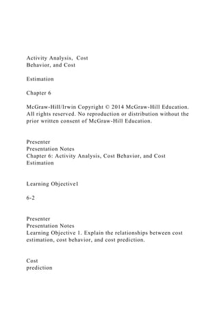
 Visual-Fit Method Vertical distance is total cost, approximately $16,000. 0 1 2 3 4 * To ta l C os t i n 1, 00 0’ s of D ol la
  • 29. rs 10 20 0 * * * * * * * * * Activity, 1,000’s of Units Produced Estimated fixed cost = $10,000 6-29 Presenter Presentation Notes The point where the line crosses the vertical axis is the estimated fixed costs. The horizontal axis is the level of activity. The vertical distance between the horizontal axis and the plotted line is the total cost at that level of activity. (LO5) The High-Low Method Owl Co recorded the following production activity &
  • 30. maintenance costs for two months: Using these two levels of activity, compute: the variable cost per unit. the total fixed cost. Units Cost High activity level 9,000 9,700$ Low activity level 5,000 6,100 6-30 Presenter Presentation Notes In the high-low method, the semi-variable cost approximation is computed using exactly two data points. The high and low activity levels are chosen from the available data set. These activity levels, together with their associated cost levels, are used to compute the variable cost per unit and the total fixed cost. (LO5) Units Cost
  • 31. High activity level 9,000 9,700$ Low activity level 5,000 6,100 Change 4,000 3,600$ The High-Low Method 6-31 Presenter Presentation Notes Before you can get started you must first calculate the change or difference in units and in cost. (LO5) Units Cost High activity level 9,000 9,700$ Low activity level 5,000 6,100 Change 4,000 3,600$ Unit variable cost = The High-Low Method 6-32 Presenter Presentation Notes The first step of the high-low method is to divide the change in cost by the change in units. (LO5) Units Cost
  • 32. High activity level 9,000 9,700$ Low activity level 5,000 6,100 Change 4,000 3,600$ Unit variable cost = $3,600 ÷ 4,000 units = $0.90 per unit The High-Low Method 6-33 Presenter Presentation Notes This will give you the variable cost per unit. (LO5) Units Cost High activity level 9,000 9,700$ Low activity level 5,000 6,100 Change 4,000 3,600$ Unit variable cost = $3,600 ÷ 4,000 units = $0.90 per unit Fixed cost = Total cost – Total variable cost The High-Low Method 6-34 Presenter Presentation Notes The next step is to determine the fixed costs. (LO5) Unit variable cost = $3,600 ÷ 4,000 units = $0.90 per unit Fixed cost = Total cost – Total variable cost
  • 33. Fixed cost = $9,700 – ($0.90 per unit × 9,000 units) Units Cost High activity level 9,000 9,700$ Low activity level 5,000 6,100 Change 4,000 3,600$ The High-Low Method 6-35 Presenter Presentation Notes The total variable cost at either the high or low level is deducted from the total cost at the same level. The total variable cost is calculated by multiplying the variable cost per unit (from step one) by the number of units. (LO5) Units Cost High activity level 9,000 9,700$ Low activity level 5,000 6,100 Change 4,000 3,600$ Unit variable cost = $3,600 ÷ 4,000 units = $.90 per unit Fixed cost = Total cost – Total variable cost Fixed cost = $9,700 – ($.90 per unit × 9,000 units) Fixed cost = $9,700 – $8,100 = $1,600 The High-Low Method 6-36
  • 34. Presenter Presentation Notes The total variable costs are deducted from the total cost to arrive at the fixed costs, $1,600. (LO5) Least-Squares Regression Method Regression is a statistical procedure used to determine the relationship between variables such as activity and cost. Activity To ta l C os t The objective of the regression method is the general cost equation: Y = a + bX 6-37 Presenter Presentation Notes Statistical techniques may be used to estimate objectively a cost behavior pattern using all of the available data.
  • 35. The most common of these methods is called least-squares regression. In the least-squares regression method, the objective is the general cost equation, Y = a + bX. (LO5) Y = a + bX Total Cost is the dependent variable. The activity (X) is the independent variable. The X term coefficient (b) is the estimate of variable cost per unit of activity, the slope of the cost line. The intercept term (a) is the estimate of fixed costs. Equation Form of Least-Squares Regression Line 6-38 Presenter Presentation Notes In the equation, X denotes the independent variable, such as activity level for a month, and Y denotes the estimated total
  • 36. utilities cost for that level of activity. The intercept of the line on the vertical axis is denoted by a, and the slope of the line is denoted by b. Within the relevant range, a is interpreted as an estimate of the fixed cost component, and b is interpreted as an estimate of the variable cost per unit of activity. In regression analysis, X is referred to as the independent variable, since it is the variable upon which the estimate is based. Y is called the dependent variable, since its estimate depends on the independent variable. (LO5) Least-Squares Regression Method courses deal with detailed regression computations using Microsoft Excel. be able to interpret and use regression estimates. 6-39 Presenter Presentation Notes The least-squares regression method does require considerably more computation than either the visual-fit or high-low method. However, computer programs are readily available to perform least-squares regression. In addition, accountants and managers must be trained to interpret and use regression estimates. (LO5)
  • 37. Learning Objective 6 6-40 Presenter Presentation Notes Learning Objective 6. Describe the multiple regression, engineering, and learning-curve approaches to cost estimation. Terms in the equation have the same meaning as in simple regression with only one independent variable. Multiple Regression Multiple regression includes two or more independent variables: Y = a + b1X1 + b2X2 6-41 Presenter Presentation Notes Multiple regression is a statistical method that estimates a linear (straight-line) relationship between one dependent variable and two or more independent variables. In a multiple regression equation, a denotes the regression estimate of the fixed-cost component, b1 denotes the regression
  • 38. estimate of the variable cost of variable 1 and b2 denotes the regression estimate of the variable cost of variable 2. The multiple-regression equation will likely enable a controller to make more accurate cost predictions than could be made with the simple regression. (LO6) Engineering Method of Cost Estimation Cost estimates are based on measurement and pricing of the work involved. 6-42 Presenter Presentation Notes A completely different method of cost estimation is to study the process that results in cost incurrence. This approach is called the engineering method of cost estimation. Engineering cost studies are time-consuming and expensive, but they often provide highly accurate estimates of cost behavior. Moreover, in rapidly evolving, high-technology industries, there may not be any historical data on which to base cost estimates. Such industries as genetic engineering, superconductivity, and electronics are evolving so rapidly that historical data are often irrelevant in estimating costs. (LO6) Direct Labor
  • 39. •Material required for each unit is obtained from engineering drawings and specification sheets. •Material prices are determined from vendor bids. •Analyze the kind of work performed. •Estimate the time required for each labor skill for each unit. •Use local wage rates to obtain labor cost per unit. Direct Material Engineering Method of Cost Estimation 6-43 Presenter Presentation Notes In a manufacturing firm, for example, a detailed study is made
  • 40. of the production technology, materials, and labor used in the manufacturing process. Rather than asking what the cost of material was last period, the engineering approach is to ask how much material should be needed and how much it should cost. Industrial engineers sometimes perform time and motion studies, which determine the steps required for people to perform the manual tasks that are part of the production process. Cost behavior patterns for various types of costs are then estimated on the basis of the engineering analysis. (LO6) Effect of Learning on Cost Behavior As I make more of these things it takes me less time for each one. It must be the learning curve effect that the boss was talking about. I’ve noticed the same thing. And if you include all the variable overhead costs that are also declining, that must be the experience curve. 6-44 Presenter Presentation Notes
  • 41. In many production processes, production efficiency increases with experience. As cumulative production output increases, the average labor time required per unit declines. As the labor time declines, labor cost declines as well. This phenomenon is called the learning curve. When the learning-curve concept is applied to a broader set of costs than just labor costs, it is referred to as an experience curve. The learning curve and experience curve concepts have been applied primarily to complex, labor-intensive manufacturing operations, such as aircraft assembly and shipbuilding. Boeing and Airbus, for example, make extensive use of the learning and experience curve concepts when budgeting the cost for a new aircraft design. However, the learning curve also has seen limited application in the health care services industry, mainly focusing on complex surgical procedures. (LO6) Learning Curve Cumulative Production Output A ve ra ge L ab or
  • 42. Ti m e pe r U ni t Learning effects are large initially. Learning effects become smaller, eventually reaching steady state. 6-45 Presenter Presentation Notes A learning curve, then, is a graphical expression of the decline in the average labor cost required per unit as cumulative output increases. Initially, the effects of learning are large. But eventually, these effects become smaller. These cost predictions are then used in scheduling production, budgeting, setting product prices, and other managerial decisions. (LO6)
  • 43. Learning Objective 7 6-46 Presenter Presentation Notes Learning Objective 7. Describe some problems often encountered in collecting data for cost estimation. Data Collection Problems 1. Missing data. 2. Outlier data points. 3. Mismatched time periods costs. 4. Trade-offs in choosing the time period. 5. Allocated and discretionary costs. 6. Inflation. 6-47 Presenter Presentation Notes Regardless of the method used, the resulting cost estimation will be only as good as the data upon which it is based. The collection of data appropriate for cost estimation requires a skilled and experienced cost analyst. Six problems frequently complicate the process of data collection: 1. Missing data.
  • 44. 2. Outliers, which could represent errors or highly unusual circumstances. 3. Mismatched time periods. 4. Trade-offs in choosing the time period. 5. Allocated and discretionary costs. 6. Inflation. (LO7) End of Chapter 6 6-48 Chapter 6Learning Objective1IntroductionLearning Objective 2Total Variable Cost ExampleVariable Cost Per Unit ExampleStep-Variable CostsStep-Variable CostsTotal Fixed Cost ExampleFixed Cost Per Unit ExampleStep-Fixed CostsStep-Fixed CostsStep-Fixed CostsSemivariable Cost Semivariable Cost Curvilinear CostLearning Objective 3Curvilinear CostLearning Objective 4Engineered, Committed, and Discretionary CostsCost Behavior in Other IndustriesCost Behavior in Other IndustriesLearning Objective 5Cost EstimationAccount Classification MethodVisual-Fit MethodSlide Number 27Slide Number 28Slide Number 29The High-Low MethodSlide Number 31Slide Number 32Slide Number 33Slide Number 34Slide Number 35Slide Number 36Least-Squares Regression MethodEquation Form of Least- Squares Regression LineLeast-Squares Regression MethodLearning Objective 6Multiple RegressionEngineering Method�of Cost EstimationEngineering Method�of Cost EstimationEffect of Learning�on Cost BehaviorLearning CurveLearning Objective 7Data Collection ProblemsEnd of Chapter 6