My first technical paper and it's on accelerated degradation modeling. My entry to reliability engineering. Engineering degradation tests allow industry to assess the potential life span of long-life products that do not fail readily under accelerated conditions in life tests. A general statistical model is presented here for performance degradation of an item of equipment. The degradation process in the model is taken to be a Wiener diffusion process with a time scale transformation. The model incorporates Arrhenius extrapolation for high stress testing. The lifetime of an item is defined as the time until performance deteriorates to a specified failure threshold. The model can be used to predict the lifetime of an item or the extent of degradation of an item at a specified future time. Inference methods for the model parameters, based on accelerated degradation test data, are presented. The model and inference methods are illustrated with a case application involving self-regulating heating cables. The paper also discusses a number of practical issues encountered in applications.

1. Lifetime Data Analysis, 3, 27–45 (1997)
c 1997 Kluwer Academic Publishers, Boston. Manufactured in The Netherlands.
Modelling Accelerated Degradation Data Using
Wiener Diffusion With A Time Scale Transformation
G. A. WHITMORE
Faculty of Management, McGill University, Montreal, Quebec H3A 1G5, Canada
FRED SCHENKELBERG
Hewlett-Packard Company, Vancouver, Washington 98683, U.S.A.
Received February 9, 1996; revised December 2, 1996; accepted December 20, 1996
Abstract. Engineering degradation tests allow industry to assess the potential life span of long-life products
that do not fail readily under accelerated conditions in life tests. A general statistical model is presented here for
performance degradation of an item of equipment. The degradation process in the model is taken to be a Wiener
diffusion process with a time scale transformation. The model incorporates Arrhenius extrapolation for high stress
testing. The lifetime of an item is defined as the time until performance deteriorates to a specified failure threshold.
The model can be used to predict the lifetime of an item or the extent of degradation of an item at a specified future
time. Inference methods for the model parameters, based on accelerated degradation test data, are presented. The
model and inference methods are illustrated with a case application involving self-regulating heating cables. The
paper also discusses a number of practical issues encountered in applications.
Keywords: Acceleration, Arrhenius, Degradation, Likelihood methods, Prediction, Statistical inference, Wiener
process
1. Introduction
Engineering degradation tests allow industry to assess the potential life span of long-life
products that do not fail readily under accelerated conditions in life tests. A general sta-
tistical model is presented here for performance degradation of an item of equipment. The
degradation process in the model is taken to be a Wiener diffusion process with a time scale
transformation. The model incorporates Arrhenius extrapolation for high stress testing.
The lifetime of an item is defined as the time until performance deteriorates to a specified
failure threshold. The model can be used to predict the lifetime of an item or the extent of
degradation of an item at a specified future time. Inference methods for the model param-
eters, based on accelerated degradation test data, are presented. The model and inference
methods are illustrated with a case application involving self-regulating heating cables. The
paper also discusses a number of practical issues encountered in applications.
2. Model
Most items deteriorate or degrade as they age. The items fail when their degradation reaches
a specified failure threshold. We assume that one key degradation measure governs failure
and take the statistical model for this measure to be a Wiener diffusion process {W (t)} with

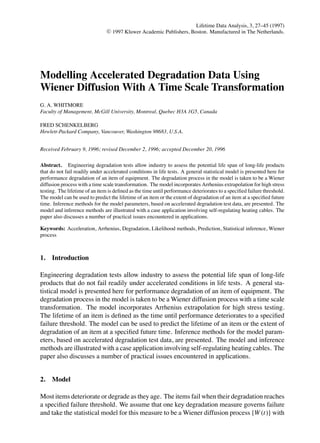
2. 28 G. A. WHITMORE AND FRED SCHENKELBERG
Figure 1. Representative sample path of a Wiener diffusion process. The path traces out the degradation of an
item over time.
mean parameter δ and variance parameter ν > 0. A Wiener process has found application
as a degradation model in other studies—see, for example, Doksum and H´ yland (1992)
o
and Lu (1995). This process represents an adequate model for the case study examined
in Section 4. Its appropriateness for general application is examined in Section 5. Basic
theoretical properties of a Wiener process may be found in Cox and Miller (1965). Figure 1
shows a representative sample path of a Wiener process. The path traces out the degradation
of an item over time, with larger values representing greater deterioration. We assume that
degradation is measured at n +1 time points ti , where t0 < t1 < · · · < tn . The measurement
at time ti is denoted by Wi = W (ti ).
The preceding Wiener model assumes that δ, the rate of degradation drift, is constant.
Where it is not constant, however, it is often found that a monotonic transformation of the
time scale can make it constant. We assume that this kind of transformation is appropriate
here and denote this transformation by
t = τ (r ), (2.1)
where r denotes the clock or calendar time and t, the transformed time. We shall require
the transformation to satisfy the initial condition τ (0) = 0. The transformed time t is often
referred to as operational time and, in physical terms, can be considered as measuring the
physical progress of degradation, such as oxidation, wearout, and so on. Because of this
physical basis for t, the transformation t = τ (r ) will depend on the particular degradation
mechanism that dominates in a given application. We shall let ti = τ (ri ) denote the
operational time corresponding to clock time ri , for i = 0, 1, . . . , n.

3. MODELLING ACCELERATED DEGRADATION DATA USING WIENER DIFFUSION 29
In the case study, we consider the following two forms of time transformation (2.1)
t = 1 − exp(−λr γ ), (2.2a)
t = r λ, (2.2b)
where both λ and γ are positive parameters. The exponential time transformation in (2.2a)
is suitable for many applications in which degradation approaches a saturation point or
asymptote where deterioration ends (for example, where oxidation ceases). The transfor-
mation has two parameters. Parameter λ usually is unknown and must be estimated in each
application. Parameter γ , on the other hand, is often a fundamental constant that is set to
some whole number or simple fractional value based on physical properties of the item. An
example of (2.2a) is found in Carey and Koenig (1991). In their case study, the propagation
delay of a logical circuit degrades (increases) along an expected path of the form (2.2a)
with γ = 1/2. Whitmore (1995) encountered a similar transformation of the time scale
in connection with the degradation of transistor gain. In his case, γ = 1. The power time
transformation in (2.2b) is suggested by the prevalence of power relationships in physical
models generally. Transformation (2.2b) implies that degradation will continue to increase
without bound. As with (2.2a), the parameter λ in (2.2b) usually must be estimated in each
application.
In developing the model in this section and the inference methodology in the following
section, we shall use time transformation (2.1) in its general form. As a final remark,
we note that Doksum and H´ yland (1992) use a similar transformed time scale to model
o
variable levels of stress in an accelerated life test. Their work prompted us to consider the
same approach in this research.
When degradation test data are gathered under accelerated or high stress conditions (such
as elevated temperature), the relation between the level of stress and the model parameters
must be established so that the parameters can be extrapolated to the lower stress conditions
encountered in actual use of the item. In our model, we have the Wiener process parameters,
δ and ν, and the parameters of the time transformation (2.1). For expository convenience,
we shall assume that the time transformation t = τ (r ) has only one parameter that is
unspecified and, hence, requires estimation. We denote this parameter by λ, as we have
done in (2.2a) and (2.2b). We then write the transformation as t = τ (r ; λ) to show the
dependence on the parameter. Both parsimony and actual experience argue for using simple
functional forms to describe the relations between the model parameters and the level of
stress. We shall let the stress be described by a single quantitative measure which we
denote by s. After applying continuous monotonic transformations to the parameters and
to the stress measure s, we assume that the relations between the transformed stress and the
transformed parameters are linear as follows.
A(δ) = a0 + a1 H (s)
B(ν) = b0 + b1 H (s) (2.3)
C(λ) = c0 + c1 H (s)
Here A(δ), B(ν), C(λ) and H (s) denote the transformations. Note that A, B and C in (2.3)
can be interpreted as a new set of parameters for the model while H can be considered as

4. 30 G. A. WHITMORE AND FRED SCHENKELBERG
a surrogate stress measure. For expository convenience, we consider only nonparametric
transformations in (2.3), such as a logarithmic or reciprocal transformation. Nonparametric
transformations are sufficient for our case study, although general applications may require
transformations with parameters that must be estimated.
The linear relationship between the log-rate of a chemical reaction and the reciprocal
absolute temperature is called the Arrhenius equation. The physical equation is widely
encountered in stress tests. As the equations in (2.3) relate the statistical parameters of
the degradation model to the level of stress, we shall refer to them here as the Arrhenius
equations and the transformation H (s) as the Arrhenius transformation. In the traditional
Arrhenius relation, H (s) = 1/s where s represents the absolute temperature in o K .
If the linear coefficients of the Arrhenius equations in (2.3) were known then reliability
predictions would proceed as follows. Given the use-level of stress, say s0 , we would
first calculate H0 = H (s0 ) and then calculate A0 = a0 + a1 H0 , B0 = b0 + b1 H0 and
C0 = c0 + c1 H0 from (2.3). Next, we would solve for the process parameters δ0 and
ν0 and the time transformation parameter λ0 under use-level conditions by inverting the
following monotonic transformations: A0 = A(δ0 ), B0 = B(ν0 ), C0 = C(λ0 ). Two kinds
of predictions could now be made.
Prediction of a Future Degradation Level
Suppose that we wish to predict the level of degradation W f at some future (clock) time r f
for a new item. We assume that the degradation measure is calibrated so a new item has
no degradation and, hence, W (0) = 0. We then exploit the fact that W f ∼ N (δ0 t f , ν0 t f )
where t f denotes the operational time corresponding to r f , i.e., t f = τ (r f ; λ0 ). This normal
distribution is the predictive distribution of W f at clock time r f under a use-level of stress.
√
Prediction limits for W f take the form δ0 t f ± z ν0 t f , where z denotes an appropriate
standard normal number.
Prediction of a Lifetime
Suppose that we wish to predict the lifetime of a new item. We must first specify a failure
threshold for the degradation process. We let ω > 0 denote this threshold level. We then
use the fact that the first passage time T to this threshold will follow the inverse Gaussian
distribution I G(ω/δ0 , ω2 /ν0 ) under use conditions (see, for example, Chhikara and Folks,
1989). The cumulative distribution function F(t) of this distribution can then be used to
make predictive statements about T . This function has the form
1 1
F(t) = (δ0 t − ω)(ν0 t)− 2 + exp(2δ0 /ν0 ) −(δ0 t + ω)(ν0 t)− 2 , (2.4)
where denotes the standard normal distribution function. It must be kept in mind here
that T refers to the operational life-time of the item under use-level conditions. The inverse
of the time transformation t = τ (r ; λ0 ) can be used to translate these predictive statements
about T into equivalent statements about the item’s lifetime measured in clock time.

5. MODELLING ACCELERATED DEGRADATION DATA USING WIENER DIFFUSION 31
3. Inference
In practice, the linear coefficients of the Arrhenius equations in (2.3) must be estimated
from accelerated degradation test data. We now give new notation to represent these test
data and specify the general characteristics of the degradation test.
We assume that m k new items are placed on test at each of K stress levels, denoted by sk ,
for k = 1, . . . , K . Let Wi jk and ri jk denote the observed degradation level and clock time,
respectively, for the ith reading on the jth item at the kth stress level. Here j = 1, . . . , m k
and i = 0, . . . , n jk . Thus, m k is the number of items on test at the kth stress level and
n jk + 1 is the number of observations made on the jth item at that stress level. We assume
that n jk ≥ 2 for each item so that the data are sufficient for parameter estimation.
We use the method of maximum likelihood to estimate the parameters δ, ν and λ for each
ˆ ˆ ˆ
item. Let these estimates be denoted by (δ jk , ν jk , λ jk ) for the jth item at the kth stress level.
To describe the estimation method, we will suppress the subscripts j and k and focus on
the n + 1 observations (Wi , ri ), i = 0, 1, . . . , n, made on an individual item. Because non-
overlapping increments in a Wiener process are independent, we consider first differences
of the observations. For i = 1, 2, . . . , n, define Wi = Wi − Wi−1 and ti = ti − ti−1 ,
where ti = τ (ri ; λ). The dependence of the differences ti on the unknown parameter λ is
suppressed in this notation. As we have
Wi ∼ N (δ ti , ν ti ), (3.1)
the sample likelihood function is
n n
1 1 ( Wi − δ ti )2
L(δ, ν, λ) = (2πν ti )− 2 exp − . (3.2)
i=1
2ν i=1
ti
By basing the sample likelihood function on first differences, the initial observation W0 =
W (t0 ) does not appear explicitly in the function. For the case study in Section 4, the initial
observation for an item is independent of the degradation process parameters and, hence, no
information is lost by omitting this initial reading from the likelihood. In some applications,
there may be a need to model the initial reading and include it in the inference structure.
The likelihood function (3.2) can be maximized directly by using a three-dimensional nu-
merical optimization routine (the approach used in the case study). An alternative approach
is to fix λ initially and then maximize the likelihood function (3.2) with respect to δ and
ν. This optimization yields the following conventional estimators, each being conditional
on λ.
Wn − W 0
ˆ
δ(λ) = (3.3a)
tn − t 0
1 n ˆ
[ Wi − δ(λ) ti ]2
ν (λ) =
ˆ (3.3b)
n i=1
ti

6. 32 G. A. WHITMORE AND FRED SCHENKELBERG
Substituting these conditional estimators back into (3.2) and simplifying, we obtain the
following partially maximized profile likelihood function.
n
n 1
L(λ) = [2π ν(λ)]− 2
ˆ ( ti )− 2 exp(−n/2) (3.4)
i=1
Recall that ti here is a function of λ. The function in (3.4) can be maximized using a
one-dimensional search over λ, yielding the maximum likelihood estimate λ. Substitution ˆ
of this estimate into each of (3.3a) and (3.3b) yields the unconditional maximum likelihood
ˆ
estimates, δ and ν . ˆ
By one of the preceding numerical methods, therefore, we obtain the triplet of parameter
ˆ ˆ ˆ
estimates (δ jk , ν jk , λ jk ) for the jth item at the kth stress level. Continuing to assume that the
transformations A, B, C and H are known for the moment, we can compute the transformed
ˆ ˆ
statistics A jk = A(δ jk ), Bjk = B(ˆ jk ), C jk = C(λ jk ), and Hk = H (sk ), for all j and k.
ν
The exact multivariate distribution of the triplets Y jk = (A jk , Bjk , C jk ) is unknown,
although we know from likelihood theory that they will be asymptotically trivariate normal.
Thus, if we let Xk = (1, Hk ) and
a0 b0 c0
B=
a1 b1 c1
then we know that
Y jk ∼ approx. N3 (Xk B, Σk ), (3.5)
where Σk denotes the covariance matrix of the triplet for each item at stress level k. Using
(3.5), the linear coefficients of the Arrhenius equations (2.3) can be estimated by multivariate
regression of the triplets Y jk on the values of Hk (see Johnson and Wichern, 1992, page
314). This regression must take account of the heteroscedastic error structure reflected in
the covariance matrix Σk . The precise form of the covariance matrix will vary from one
application to another. The regression analysis is illustrated in Section 4.
Once the estimated Arrhenius equations are available, the predictive analysis described in
the preceding section can be applied, provided two remaining hurdles are overcome. First,
account must be taken of the sampling errors in the estimated coefficients in (2.3) when
they are used for predictive analysis. Second, the correct transformations A(δ), B(ν), C(λ)
and H (s) must be identified. These two hurdles need to be dealt with on a case-by-case
basis.
In some applications, the sampling errors in the estimated coefficients of (2.3) represent
effects of secondary importance and, hence, can be ignored in predictive analysis. Where
the sampling errors will have a material effect on predictive statements, a strategy is needed
to take their effect into account. Development of exact analytical results appears to be
infeasible. A practical approach might employ sensitivity analysis, simulation or a Bayesian
procedure; these methods being in increasing order of sophistication. The estimator of the
coefficient matrix B in regression model (3.5) is the key input to predictions. The estimator,
ˆ
which we denote by B, has an asymptotic multivariate normal distribution that can be
estimated using conventional regression theory. The estimated distribution can then be

7. MODELLING ACCELERATED DEGRADATION DATA USING WIENER DIFFUSION 33
used to set the parameter ranges for a simple sensitivity analysis. It can also be used to
construct composite prediction intervals for a future degradation level W f or the lifetime T
of an item by generating simulated outcomes of B. Finally, the asymptotic distribution can
be used to calculate Bayesian prediction intervals.
Identifying the correct transformations A(δ), B(ν), C(λ) and H (s) can be approached by
using a combination of subject matter knowledge and statistical procedures. The subject
matter may suggest, for example, that H (s) has the Arrhenius form mentioned earlier. The
subject matter may also suggest forms for A(δ), B(ν) and C(λ). Candidate transformations
might also be identified by examining appropriate graphs, backed up by formal goodness-
of-fit tests. To illustrate the fitting approach for A(δ), we note that there are m k observations
A jk , j = 1, . . . , m k , at each stress level sk . Hence, an ANOVA test of linearity may be used,
based on sums of squares for pure error and lack of fit. This technique will be demonstrated
in the case study presented in the next section.
4. Case Application
The Chemelex Division of the Raychem Corporation in Redwood City, California makes
a self-regulating heating cable that finds extensive application in conditions that require
high reliability. These cables are subjected to extensive degradation testing, both to ensure
the dependability of current products and to support the development of new and improved
product designs. The data set presented in this case study is a disguised version of a typical
test set. The disguise does not alter the essential statistical properties being studied but does
protect the proprietary interests of the company.
The test items in this case application are sample cable lengths cut from a production
lot. Degradation of the cable is indicated by a rise in its electrical resistance with age. We
shall use the natural logarithm of resistance as the degradation measure W . Degradation of
the cable is accelerated by thermal stress so temperature (measured in ◦ K ) is used as the
stress measure. The test data consist of readings on log-resistance at several time points for
each item. The readings of log-resistance are standardized to 0 at time r = 0 to adjust for
small differences in the cable lengths of the items. This type of cable experiences a slight
improvement in performance (i.e., a drop in resistance) when it is first placed in operation.
This initial improvement is attributed to curing of the cable polymer. For this reason, only
degradation readings taken subsequent to this cure phase are considered for the analysis.
Five test items were baked in an oven at each test temperature. Three test temperatures
were used, 200◦ C, 240◦ C, 260◦ C, giving a total of 15 test items. Ten readings were recorded
after the cure phase on each item tested at 200◦ C. Similarly, 11 readings were recorded on
each of four items tested at 240◦ C. Only 10 readings were available for the 5th item tested
at this temperature. The last reading is missing because of a test fixture failure. Finally,
seven readings were recorded on each item tested at 260◦ C. The test data appear in Table 1.
The clock times in the table are in thousands of hours.
The test design and protocol are based on an internal company specification. The selected
temperature levels and number of items tested at each temperature were determined by the
limitations of available test equipment and the logistics of handling test fixtures. The
temperature levels were chosen to span the range from the maximum level that would be

8. 34 G. A. WHITMORE AND FRED SCHENKELBERG
Table 1. Heating cable test data. Degradation is measured as the natural logarithm
of resistance. Time is measured in thousands of hours. A period denotes a missing
value.
Item
Time 1 2 3 4 5
(a) Test temperature 200◦ C.
0.496 −0.120682 −0.118779 −0.123600 −0.126501 −0.124359
0.688 −0.112403 −0.109853 −0.115186 −0.118941 −0.111966
0.856 −0.103608 −0.101593 −0.105657 −0.110288 −0.107869
1.024 −0.096047 −0.094567 −0.098569 −0.103419 −0.100304
1.192 −0.085673 −0.084698 −0.088613 −0.095465 −0.085916
1.360 −0.077677 −0.076070 −0.079332 −0.084769 −0.077947
2.008 −0.045218 −0.040623 −0.045835 −0.052268 −0.045597
2.992 0.000526 0.004237 0.000533 −0.008265 0.000524
4.456 0.059261 0.063742 0.061032 0.051139 0.059544
5.608 0.093394 0.095117 0.093612 0.082414 0.084912
(b) Test temperature 240◦ C.
0.160 −0.005152 −0.019888 −0.045961 −0.023188 −0.044267
0.328 0.056930 0.046278 0.015198 0.040737 0.018173
0.496 0.112631 0.101628 0.067119 0.095504 0.072214
0.688 0.173202 0.162705 0.128670 0.156129 0.131555
0.856 0.214266 0.202604 0.168271 0.196349 0.171394
1.024 0.272668 0.257563 0.221611 0.250900 0.225281
1.192 0.311422 0.297875 0.260910 0.291937 0.266314
1.360 0.351988 0.338902 0.302126 0.332887 0.306105
2.008 0.489847 0.461855 0.440738 0.473130 0.443941
2.992 0.656780 0.629991 0.606275 0.638651 0.611724
4.456 0.851985 0.798431 0.834114 0.798457 .
(c) Test temperature 260◦ C.
0.160 0.123360 0.127605 0.120759 0.105206 0.120115
0.328 0.251084 0.254944 0.247156 0.232389 0.247949
0.496 0.393107 0.394496 0.391516 0.375789 0.388406
0.688 0.517137 0.518485 0.513872 0.500556 0.511850
0.856 0.598797 0.599265 0.595704 0.583362 0.595220
1.024 0.693925 0.694445 0.688930 0.679117 0.690324
1.192 0.774347 0.774428 0.770313 0.758314 0.770782
encountered in field installations to a level where the cable polymer undergoes a physical
phase change. The earliest test readings were made at roughly weekly intervals, with
the interval lengthening for later readings. The test was discontinued when the test items
went through the failure threshold for the 240◦ C and 260◦ C test temperatures. According to
company specifications, the cable is deemed to have failed when the resistance doubles (i.e.,

9. MODELLING ACCELERATED DEGRADATION DATA USING WIENER DIFFUSION 35
the log-resistance reaches ln(2) = 0.693). The test continued at the lowest test temperature
(200◦ C) until the test equipment was required for other projects.
Both forms of the time transformation given in (2.2) were used in the study. Once the
analyses were completed and the final results were in hand, company scientists found reasons
to prefer one transformation over the other based on scientific considerations. Still, some
uncertainty about the appropriate transformation remains which only additional empirical
evidence can eliminate. It is instructive to compare the two sets of results that the scientists
had to consider. We begin with the results for transformation (2.2a).
Exponential Time Transformation
The NONLIN procedure of the statistical software package SYSTAT was used to obtain
ˆ ˆ ˆ
the estimates (δ jk , ν jk , λ jk ) for the jth item ( j = 1, . . . , 5) at the kth temperature level
(k = 1, 2, 3) by maximizing the sample likelihood function (3.2) for each of the 15 items.
The exponential time transformation (2.2a) was used in this application of the maximum
likelihood method with the parameter γ set to 1. Thus, in setting up the sample likelihood
function (3.2), each clock time was transformed as follows.
ti jk = 1 − exp(−λri jk )
The parameter estimates for each of the items appear in Table 2. The results show that the
parameter estimates are reasonably consistent across items at each temperature level. Two
exceptions might be item 5 at test temperature 200◦ C and item 3 at test temperature 240◦ C.
The findings presented here are based on the whole data set because there was no external
reason to believe that either of these two outlying points is invalid or unrepresentative.
Each set of parameter estimates was plotted against the reciprocal of the absolute temper-
ature. Based on these three plots, the following parameter transformations were tentatively
identified.
A(δ) = δ, B(ν) = ln(ν), C(λ) = 1/λ (4.1)
The plots for the transformed parameters appear in Figure 2. Consultations with company
scientists revealed that little was known of the statistical properties of the physical degra-
dation mechanism. It was therefore difficult to judge whether these transformations were
reasonable from a scientific point of view. Thus, the final judgment was to be based on the
adequacy of the statistical fit, which we return to describe shortly.
The plots in Figure 2 show roughly linear relationships but also exhibit patterns of het-
eroscedasticity that need to be accommodated. It was especially noted in the plots for ln(ν) ˆ
ˆ
and 1/λ in Figures 2b and 2c that the scatter of points shrinks as the reciprocal temperature
decreases (i.e., as the temperature increases). In fact, it seems that the variability vanishes
just above the highest test temperature at 260◦ C or 533◦ K , where 1/s3 = 0.001876. We
have already mentioned that the cable polymer experiences a phase change near this tem-
perature level. As the resistance properties of the polymer are altered by the phase change,
it was suspected that this factor might explain why the variability of resistance readings

10. 36 G. A. WHITMORE AND FRED SCHENKELBERG
Table 2. Parameter estimates for all test items based on the exponential time
transformation.
(a) Test temperature 200◦ C
Parameter Item
Estimate 1 2 3 4 5
ˆ
δ 0.495231 0.454562 0.474481 0.473190 0.378924
ˆ
λ 0.120107 0.137024 0.131168 0.124015 0.181333
ˆ
ν 0.000094 0.000129 0.000122 0.000170 0.000398
(b) Test temperature 240◦ C
Parameter Item
Estimate 1 2 3 4 5
ˆ
δ 1.278160 1.145816 1.478103 1.130811 1.157966
ˆ
λ 0.281411 0.324826 0.223447 0.339209 0.320289
ˆ
ν 0.000898 0.000819 0.001357 0.000423 0.000470
(c) Test temperature 260◦ C
Parameter Item
Estimate 1 2 3 4 5
ˆ
δ 1.491041 1.492564 1.482068 1.485528 1.506090
ˆ
λ 0.640612 0.632789 0.644703 0.648073 0.629577
ˆ
ν 0.001701 0.001618 0.001876 0.001740 0.001467
converged to zero upon approaching this critical temperature. We shall denote this criti-
cal temperature by sc and set it to 535◦ K . The patterns of heteroscedasticity in the three
plots therefore suggested that the following scaled version of the Arrhenius transformation
should be considered.
1 1
H (s) = − for s ≤ sc (4.2)
s sc
Observe that H (s) in (4.2) is a decreasing function of s with H (sc ) = 0. The patterns of
heteroscedasticity suggest therefore that the appropriate form for the covariance matrix in
(3.5) is
Σk = Hk Σ, (4.3)
where Hk = H (sk ) is based on the function in (4.2) and Σ denotes a baseline covariance
matrix that is common to all items. A statistical software routine for weighted multivariate
regression may now be used to estimate the coefficient matrix B in (3.5) and covariance
matrix Σ in (4.3), using the reciprocals of the Hk values as weights.

11. MODELLING ACCELERATED DEGRADATION DATA USING WIENER DIFFUSION 37
(a) Estimates of A(δ) = δ. (b) Estimates of B(ν) = ln(ν).
(c) Estimates of C(λ) = 1/λ.
Figure 2. Plots of the transformed parameter estimates against the reciprocal of the test temperature (in ◦ K ) for
each test item, based on the exponential time transformation t = 1 − exp(−λr ).
The result in (4.3) implies that the following transformations will yield a set of centered
quantities with a stable variance at each temperature level sk .
A jk − a0 − a1 Hk
A jk = √ (4.4a)
Hk

12. 38 G. A. WHITMORE AND FRED SCHENKELBERG
Bjk − b0 − b1 Hk
B jk = √ (4.4b)
Hk
C jk − c0 − c1 Hk
C jk = √ (4.4c)
Hk
The pairs of regression coefficients, (a0 , a1 ), (b0 , b1 ) and (c0 , c1 ), can also be estimated
directly from the quantities in (4.4) by minimizing the total sum of squares for each of the
three sets of values. The resulting estimates of the Arrhenius equations are
ˆ
δ = 1.5237 − 4173.0H (s), (4.5a)
ln(ˆ = −6.3255 − 10, 224H (s),
ν) (4.5b)
ˆ
1/λ = 1.3961 + 24, 617H (s), (4.5c)
where H (s) is defined as in (4.2) with sc = 535.
An ANOVA test for linearity was performed for each parametric transformation in (4.1)
based on the three sets of quantities in (4.4). First, taking the A jk values in (4.4a), a
Hartley test for equal population variances at each of the three test temperature levels
was performed (Neter, Wasserman and Kutner, 1990, page 619), yielding a test statistic
of H = 5.680. The 0.95 fractile of H under the null hypothesis is 15.5 which suggests
that the hypothesis of equal variances cannot be rejected. Next, the centered total sum of
squares of the quantities A jk was decomposed into component sums of squares relating to
within and between temperature-level variation, respectively. The P- value of the resulting
ANOVA test was 0.389, which is not significant. Similar tests were conducted for B jk and
C jk . Their H statistics were 1.564 and 10.874, and the P-values for their ANOVA tests
were 0.846 and 0.948, respectively. None of these test results is significant. Thus, the
tests support the conclusion that each parameter transformation in (4.1) produces a linear
Arrhenius equation.
Power Time Transformation
The same analysis as just described was repeated using the power time transformation (2.2b)
in lieu of the exponential time transformation. In setting up the sample likelihood function
(3.2), each clock time was transformed as follows.
ti jk = riλjk
Table 3 contains the maximum likelihood estimates of the parameters δ, ν and λ for each
item. Although the parameter symbols are the same as for the exponential time transfor-
mation, their interpretation is different. Parameter λ here denotes the power parameter
in the time transformation. The drift parameter δ and variance parameter ν now relate to

13. MODELLING ACCELERATED DEGRADATION DATA USING WIENER DIFFUSION 39
Table 3. Parameter estimates for all test items based on the power time
transformation.
(a) Test temperature 200◦ C
Parameter Item
Estimate 1 2 3 4 5
ˆ
δ 0.067033 0.070529 0.070460 0.064614 0.083440
ˆ
λ 0.770625 0.746937 0.754399 0.776336 0.662939
ˆ
ν 0.000026 0.000039 0.000035 0.000039 0.000120
(b) Test temperature 240◦ C
Parameter Item
Estimate 1 2 3 4 5
ˆ
δ 0.402380 0.425770 0.367597 0.427560 0.369068
ˆ
λ 0.6028l7 0.553013 0.662507 0.552947 0.665162
ˆ
ν 0.000442 0.000523 0.000229 0.000753 0.000214
(c) Test temperature 260◦ C
Parameter Item
Estimate 1 2 3 4 5
ˆ
δ 0.788621 0.781160 0.788423 0.791786 0.784428
ˆ
λ 0.661233 0.664679 0.659068 0.660399 0.666644
ˆ
ν 0.001172 0.001096 0.001283 0.001255 0.001017
a different operational time scale. The results in Table 3 again show that the parameter
estimates are reasonably consistent across items at each temperature level. Item 5 at test
temperature 200◦ C and item 3 at 240◦ C remain somewhat outlying, as does item 5 at 240◦ C.
The analysis continues to be based on the whole data set, however, because there was no
external reason to believe that any of these outlying points is invalid or unrepresentative.
Each set of parameter estimates was plotted against the reciprocal of the absolute temper-
ature. Based on two of these plots, the following parameter transformations were tentatively
identified.
A(δ) = ln(δ), B(ν) = ln(ν) (4.6)
The plots for the transformed parameters are shown in Figures 3a and 3b. The two plots
appear to be nearly linear. An appropriate transformation for λ could not be identified.
ˆ ˆ
Figure 3c shows a plot of λ against the reciprocal temperature. The value of λ appears to
◦
be lowest at the intermediate reciprocal-temperature level (240 C) and distinctly elevated
at the highest reciprocal-temperature level (200◦ C).

14. 40 G. A. WHITMORE AND FRED SCHENKELBERG
(a) Estimates of A(δ) = ln(δ). (b) Estimates of B(ν) = ln(ν).
(c) Estimates of λ (untransformed).
Figure 3. Plots of the transformed parameter estimates against the reciprocal of the test temperature (in ◦ K ) for
each test item, based on the power time transformation t = r λ .
To explore the parameter λ further, we have computed the combined profile log-likelihood
function ln L k (λ) for all items tested at temperature level sk , as follows.
mk
ln L k (λ) = ln L jk (λ) for k = 1, 2, 3 (4.7)
j=1

15. MODELLING ACCELERATED DEGRADATION DATA USING WIENER DIFFUSION 41
Figure 4. Plot of the combined profile log-likelihood function ln L k (λ) for all items on test at each test temperature
sk . The vertical scale measures the decrement from the maximum log-likelihood level for each function.
Here L jk (λ) denotes the profile likelihood function of form (3.4) for the jth item tested
at temperature sk . Figure 4 shows a plot of this combined profile log-likelihood function
for each temperature level. The vertical scale measures the decrement from the maximum
log-likelihood level. The functions are close to being quadratic in shape. From likelihood
theory we know that the interval spanned by each function at a decrement of −1.92 from the
maximum log-likelihood is an approximate 95% confidence interval for λ at that temperature
level. The intervals suggest that parameter λ is larger at 200◦ C than at 240◦ C, with the
parameter taking an intermediate value at 260◦ C. Thus, both Figure 3c and Figure 4 suggest
that λ is not related to temperature in a monotonic fashion.
The plots in Figure 3 show patterns of heteroscedasticity that are similar to those seen
in Figure 2. We therefore employ the same Arrhenius transformation as in (4.2). The
critical temperature for this transformation remains at sc = 535◦ K . The estimation of the
Arrhenius equations proceeds as with the exponential time transformation except that we
will omit the estimation of c0 and c1 for the equation involving λ because we cannot decide

16. 42 G. A. WHITMORE AND FRED SCHENKELBERG
on the appropriate form for the transformation C(λ). The resulting estimated Arrhenius
equations are as follows
ˆ
ln(δ) = −0.16728 − 9952.8H (s), (4.7a)
ln(ˆ ) = −6.6652 − 14, 011H (s),
ν (4.7b)
where H (s) is defined as in (4.2) with sc = 535.
ANOVA tests for linearity, together with Hartley tests for equal variances, indicate that the
parameter transformations in (4.6) yield linear Arrhenius equations. The Hartley statistics
are H = 4.159 and H = 1.669 and the ANOVA P-values are 0.175 and 0.905, respectively.
The statistical analyses based on the two forms of the time transformation have yielded
results that are comparable in terms of the fit of the model to the data. We now look at how
company scientists weighed the competing results.
Oxidation of the cable polymer is considered to be the principal degradation mechanism.
If oxidation were a self-limiting reaction then the exponential time transformation might
be appropriate. Company scientists did not rule out this self-limiting feature. However,
if oxidation is self-limiting then the asymptotic log-resistance of the cable would have
an expected value of δ, corresponding to r = ∞ or t = 1. The Arrhenius equation
A(δ) = a0 +a1 H (s) fitted under the exponential time transformation—see (4.5a)—indicates
that δ varies with the test temperature, which implies that the asymptotic log-resistance
varies with the aging temperature. Company scientists felt that this feature was implausible
although there is no empirical evidence based on long aging studies to settle the question.
Hence, the implications of the exponential time transformation were unacceptable. The
behaviour of the model based on the power time transformation was more satisfactory to
the scientists. Interestingly, the transformations A(δ) and B(ν) were both of a logarithmic
form which was a satisfying feature. The power transformation also implied that the log-
resistance would rise without limit as the cable aged, which was a plausible behavior.
The uncertainty about the form of the Arrhenius equation for the power parameter λ was a
difficulty but the fact that the estimates of λ had only a small range of values was reassuring.
Further testing is being planned that might settle the question of the appropriate form for
C(λ). In summary, company scientists felt more comfortable with the implications of the
power time transformation.
We now look at predictive inference for the power transformation model. Recall that the
cable is deemed to have failed when the resistance doubles. Thus, ω = ln(2) = 0.69315.
The normal use temperature of the cable is 175◦ C, which gives s0 = 448◦ K . At this
temperature, we have
1 1 1 1
H0 = − = − = 0.0003630.
s0 sc 448 535
The Arrhenius equations in (4.7a) and (4.7b) give the following results.
ˆ
ln(δ0 ) = −0.16728 − 9952.8(0.0003630) = −3.780
ln(ˆ 0 ) = −6.6652 − 14, 011(0.0003630) = −11.751
ν

17. MODELLING ACCELERATED DEGRADATION DATA USING WIENER DIFFUSION 43
Thus, the corresponding use-level parameter estimates are
ˆ
δ0 = exp(−3.780) = 0.02282,
ν0 = exp(−11.751) = 0.7883 × 10−5 .
ˆ
The use-level estimate of λ0 is still required and, as we saw in Figure 3c, it is unclear how
to extrapolate the test results to obtain this estimate. Rather than attempt an estimate, we
carry out a sensitivity analysis. We wish to calculate the probability that the resistance of a
new item will double within, say, its first 10 years of life. We must first convert this clock
time to operational time using the transformation t f = 87.6λ0 , where r f = 87.6 thousand
hours corresponds to 10 years. Taking a range of plausible values for λ0 and ignoring
the sampling errors in the other parameter estimates, we use the cumulative distribution
function in (2.4) with t = t f to calculate the required failure probability. The following
table gives this failure probability for part of the range of λ0 values of interest.
λ0 : 0.74 0.75 0.76 0.77 0.78
P(T ≤ t f ): 0.0000 0.0042 0.2629 0.9145 0.9996
The table shows that the failure probability is very sensitive to λ0 in this part of the range,
varying from 0 to near 1 in a short interval. The sensitivity analysis suggests that the failure
probability is small only if λ0 is below 0.75. As 200◦ C is the test temperature that is closest
to the use-level temperature, it is instructive to look at the λ estimates for the five items that
were tested at that temperature (see Table 3a). Three of the five items have λ estimates that
are larger than the critical value 0.75 and two that are smaller—a mixed result. Thus, under
the power time transformation, this data set has not provided precise information about
the 10-year failure probability for this product. As already mentioned, further degradation
testing is being planned. This additional testing may yield a better assessment of the use-
level parameter λ0 and settle the question of the appropriate form for transformation C(λ).
As a concluding remark, we add that this kind of heating cable has proven to be very reliable
in field installations to date, which suggests that λ0 may indeed be well below the critical
value.
5. Discussion and Conclusions
The model and case study presented here have left a number of practical issues untouched.
Many of these can be dealt with by appropriate technical extensions.
Measurement errors are produced by imperfect laboratory personnel, procedures and
equipment. An extension of our model, similar to that described in Whitmore (1995), can
take measurement errors into account. In our experimental setting, however, measurement
errors are likely to be intercorrelated because readings on test items are made at the same
time under the same test conditions. For instance, in the case study, all test items in the
same oven are withdrawn together and cooled to room temperature before their resistances
are measured. They are then returned to the ovens and brought back up to test temperature.
Any measurement imperfections in this setting will affect all items in the batch.

18. 44 G. A. WHITMORE AND FRED SCHENKELBERG
A Wiener diffusion process may not describe the degradation process of interest in some
applications. For example, degradation may proceed in a strictly monotonic fashion or
involve jump behavior. In these circumstances, the Wiener process might be replaced by
a more appropriate process, such as a Hougaard process (see Lee and Whitmore, 1993,
and Fook Chong, 1993). The Hougaard family includes the gamma and inverse Gaussian
processes as special cases. Degradation may also be a multidimensional process in which
the boundary conditions that define failure are more complicated than a simple failure
threshold.
The model presented here assumes that stress s is a single quantitative measure, such
as temperature. This assumption is more restrictive than necessary. Stress s can be a
multidimensional physical measure. The model would still apply, provided a function
H (s) exists that maps each measure s into a real number. The number H (s) then becomes
a stress index for the multidimensional measure s. The challenge in this extension would
be to discover the appropriate form of the function H (s).
The scaled version of the Arrhenius transformation in (4.2) assumes that sc is the same
for all parameters and is known. In the case study, however, there is some evidence that
this critical temperature is not sharply delineated and may be a little different for different
parameters. Perhaps sc should be treated as another parameter that must be estimated for
each Arrhenius equation. This issue is one of many that demonstrate the general need for a
better understanding of the link between statistical parameters and the physical parameters
of the scientific theories that underpin each application.
The results of the case study demonstrate the need to examine the appropriate design
for degradation tests. The model provides a framework for studying design issues such as
the selection of stress levels, the number of items on test, and the number and spacings of
readings on each item. The design should aim not only to optimize predictive accuracy
but also to have a self-testing capability that would allow the model itself to be validated
through appropriate diagnostics.
Acknowledgments
This research was completed while one of the authors (Schenkelberg) was employed by the
Raychem Corporation. We thank the Corporation for permission to use the case study re-
sults. We also are deeply indebted to scientists of the Corporation for providing background
scientific information and expert opinion about the materials and degradation processes in-
volved. We thank two anonymous referees for helpful suggestions on an earlier version of
this paper. Finally, we are grateful for the financial support provided for this research by
the Natural Sciences and Engineering Research Council of Canada.
References
M. Boulanger Carey and R. H. Koenig, “Reliability assessment based on accelerated degradation: A case study,”
IEEE Transactions on Reliability vol. 40(5) pp. 499–506, 1991.
R. S. Chhikara and J. L. Folks, The Inverse Gaussian Distribution: Theory, Methodology and Applications, Marcel
Dekker: New York, 1989.

19. MODELLING ACCELERATED DEGRADATION DATA USING WIENER DIFFUSION 45
D. R. Cox and H. D. Miller. The Theory of Stochastic Processes, Chapman and Hall: London, 1965.
K. A. Doksum and A. H´ yland, “Models for variable-stress accelerated life testing experiments based on Wiener
o
processes and the inverse Gaussian distribution,” Technometrics vol. 34(1) pp. 74–82, 1992.
S. Fook Chong, A Study of Hougaard Distributions, Hougaard Processes and Applications, M.Sc. thesis, McGill
University, Montreal, 1993.
R. A. Johnson and D. W. Wichern, Applied Multivariate Statistical Analysis, 3rd edition, Prentice-Hall: Englewood
Cliffs, New Jersey, 1992.
M.-L. T. Lee and G. A. Whitmore, “Stochastic processes directed by randomized time,” Journal of Applied
Probability vol. 30 pp. 302–314, 1993.
J. Lu, A Reliability Model Based on Degradation and Lifetime Data, Ph.D. thesis, McGill University, Montreal,
Canada, 1995.
J. Neter, W. Wasserman and M. H. Kutner, Applied Linear Statistical Models, 3rd edition, Irwin: Homewood,
Illinois, 1990.
G. A. Whitmore, “Estimating degradation by a Wiener diffusion process subject to measurement error,” Lifetime
Data Analysis vol. 1(3) pp. 307–319, 1995.