Toolboxweb

A Stochastic Processes Toolkit for Risk Management∗
Damiano Brigo† Antonio Dalessandro‡ Matthias Neugebauer§ Fares Triki¶
, , ,
15 November 2007

Abstract
In risk management it is desirable to grasp the essential statistical features of a time series rep-
resenting a risk factor. This tutorial aims to introduce a number of different stochastic processes
that can help in grasping the essential features of risk factors describing different asset classes or
behaviors. This paper does not aim at being exhaustive, but gives examples and a feeling for practi-
cally implementable models allowing for stylised features in the data. The reader may also use these
models as building blocks to build more complex models, although for a number of risk management
applications the models developed here suffice for the first step in the quantitative analysis. The
broad qualitative features addressed here are fat tails and mean reversion. We give some orientation
on the initial choice of a suitable stochastic process and then explain how the process parameters
can be estimated based on historical data. Once the process has been calibrated, typically through
maximum likelihood estimation, one may simulate the risk factor and build future scenarios for the
risky portfolio. On the terminal simulated distribution of the portfolio one may then single out
several risk measures, although here we focus on the stochastic processes estimation preceding the
simulation of the risk factors Finally, this first survey report focuses on single time series. Correlation
or more generally dependence across risk factors, leading to multivariate processes modeling, will be
addressed in future work.

JEL Classification code: G32, C13, C15, C16.
AMS Classification code: 60H10, 60J60, 60J75, 65C05, 65c20, 91B70
Key words: Risk Management, Stochastic Processes, Maximum Likelihood Estimation, Fat Tails, Mean
Reversion, Monte Carlo Simulation

∗ We are grateful to Richard Hrvatin and Lars Jebjerg for reviewing the manuscript and for helpful comments. Kyr-

iakos Chourdakis furhter helped with comments and formatting issues. Contact: richard.hrvatin@fitchratings.com,
lars.jebjerg@fitchratings.com, kyriakos.chourdakis@fitchratings.com
† Fitch Solutions, and Department of Mathematics, Imperial College, London. damiano.brigo@fitchratings.com
‡ Fitch Solutions, and Department of Mathematics, Imperial College, London. antonio.dalessandro@ic.ac.uk
§ Fitch Ratings. matthias.neugebauer@fitchratings.com
¶ Fitch Solutions, and Paris School of Economics, Paris. fares.triki@fitchratings.com

1

Contents
1 Introduction 3

2 Modelling with Basic Stochastic Processes: GBM 5

3 Fat Tails: GARCH Models 13

4 Fat Tails: Jump Diﬀusion Models 17

5 Fat Tails Variance Gamma (VG) process 21

6 The Mean Reverting Behaviour 25

7 Mean Reversion: The Vasicek Model 27

8 Mean Reversion: The Exponential Vasicek Model 31

9 Mean Reversion: The CIR Model 33

10 Mean Reversion and Fat Tails together 36

2

D. Brigo, A. Dalessandro, M. Neugebauer, F. Triki: A stochastic processes toolkit for Risk Management 3

1 Introduction
In risk management and in the rating practice it is desirable to grasp the essential statistical features
of a time series representing a risk factor to begin a detailed technical analysis of the product or the
entity under scrutiny. The quantitative analysis is not the final tool, since it has to be integrated with
judgemental analysis and possible stresses, but represents a good starting point for the process leading
to the final decision.
This tutorial aims to introduce a number of different stochastic processes that, according to the
economic and financial nature of the specific risk factor, can help in grasping the essential features of
the risk factor itself. For example, a family of stochastic processes that can be suited to capture foreign
exchange behaviour might not be suited to model hedge funds or a commodity. Hence there is need
to have at one’s disposal a sufficiently large set of practically implementable stochastic processes that
may be used to address the quantitative analysis at hand to begin a risk management or rating decision
process.
This report does not aim at being exhaustive, since this would be a formidable task beyond the scope
of a survey paper. Instead, this survey gives examples and a feeling for practically implementable models
allowing for stylised features in the data. The reader may also use these models as building blocks to build
more complex models, although for a number of risk management applications the models developed here
suffice for the first step in the quantitative analysis.
The broad qualitative features addressed here are fat tails and mean reversion. This report begins
with the geometric Brownian motion (GBM) as a fundamental example of an important stochastic process
featuring neither mean reversion nor fat tails, and then it goes through generalisations featuring any of the
two properties or both of them. According to the specific situation, the different processes are formulated
either in (log-) returns space or in levels space, as is more convenient. Levels and returns can be easily
converted into each other, so this is indeed a matter of mere convenience.
This tutorial will address the following processes:

• Basic process: Arithmetic Brownian Motion (ABM, returns) or GBM (levels).
• Fat tails processes: GBM with lognormal jumps (levels), ABM with normal jumps (returns),
GARCH (returns), Variance Gamma (returns).
• Mean Reverting processes: Vasicek, CIR (levels if interest rates or spreads, or returns in
general), exponential Vasicek (levels).
• Mean Reverting processes with Fat Tails: Vasicek with jumps (levels if interest rates or
spreads, or returns in general), exponential Vasicek with jumps (levels).

Different financial time series are better described by different processes above. In general, when first
presented with a historical time series of data for a risk factor, one should decide what kind of general
properties the series features. The financial nature of the time series can give some hints at whether
mean reversion and fat tails are expected to be present or not. Interest rate processes, for example, are
often taken to be mean reverting, whereas foreign exchange series are supposed to be often fat tailed and
credit spreads feature both characteristics. In general one should:
Check for mean reversion or stationarity
Some of the tests mentioned in the report concern mean reversion. The presence of an autoregressive
(AR) feature can be tested in the data, typically on the returns of a series or on the series itself if this
is an interest rate or spread series. In linear processes with normal shocks, this amounts to checking
stationarity. If this is present, this can be a symptom for mean reversion and a mean reverting process
can be adopted as a first assumption for the data. If the AR test is rejected this means that there is
no mean reversion, at least under normal shocks and linear models, although the situation can be more
complex for nonlinear processes with possibly fat tails, where the more general notions of stationarity
and ergodicity may apply. These are not addressed in this report.
If the tests find AR features then the process is considered as mean reverting and one can compute
autocorrelation and partial autocorrelation functions to see the lag in the regression. Or one can go


directly to the continuous time model and estimate it on the data through maximum likelihood. In this
case, the main model to try is the Vasicek model.
If the tests do not find AR features then the simplest form of mean reversion for linear processes
with Gaussian shocks is to be rejected. One has to be careful though that the process could still be
mean reverting in a more general sense. In a way, there could be some sort of mean reversion even under
non-Gaussian shocks, and example of such a case are the jump-extended Vasicek or exponential Vasicek
models, where mean reversion is mixed with fat tails, as shown below in the next point.
Check for fat tails If the AR test fails, either the series is not mean reverting, or it is but with fatter
tails that the Gaussian distribution and possibly nonlinear behaviour. To test for fat tails a first graphical
tool is the QQ-plot, comparing the tails in the data with the Gaussian distribution. The QQ-plot gives
immediate graphical evidence on possible presence of fat tails. Further evidence can be collected by
considering the third and fourth sample moments, or better the skewness and excess kurtosis, to see
how the data differ from the Gaussian distribution. More rigorous tests on normality should also be
run following this preliminary analysis1. If fat tails are not found and the AR test failed, this means
that one is likely dealing with a process lacking mean reversion but with Gaussian shocks, that could be
modeled as an arithmetic Brownian motion. If fat tails are found (and the AR test has been rejected),
one may start calibration with models featuring fat tails and no mean reversion (GARCH, NGARCH,
Variance Gamma, arithmetic Brownian motion with jumps) or fat tails and mean reversion (Vasicek
with jumps, exponential Vasicek with jumps). Comparing the goodness of fit of the models may suggest
which alternative is preferable. Goodness of fit is determined again graphically through QQ-plot of the
model implied distribution against the empirical distribution, although more rigorous approaches can be
applied 2 . The predictive power can also be tested, following the calibration and the goodness of fit tests.
3
.
The above classification may be summarized in the table, where typically the referenced variable is
the return process or the process itself in case of interest rates or spreads:

Normal tails Fat tails
NO mean reversion ABM ABM+Jumps,
(N)GARCH, VG
Mean Reversion Vasicek Exponential Vasicek
CIR, Vasicek with Jumps

Once the process has been chosen and calibrated to historical data, typically through regression
or maximum likelihood estimation, one may use the process to simulate the risk factor over a given
time horizon and build future scenarios for the portfolio under examination. On the terminal simulated
distribution of the portfolio one may then single out several risk measures. This report does not focus
on the risk measures themselves but on the stochastic processes estimation preceding the simulation of
the risk factors. In case more than one model is suited to the task, one can analyze risks with different
models and compare the outputs as a way to reduce model risk.
Finally, this first survey report focuses on single time series. Correlation or more generally dependence
across risk factors, leading to multivariate processes modeling, will be addressed in future work.
Prerequisites
The following discussion assumes that the reader is familiar with basic probability theory, includ-
ing probability distributions (density and cumulative density functions, moment generating functions),
random variables and expectations. It is also assumed that the reader has some practical knowledge of
stochastic calculus and of It¯’s formula, and basic coding skills. For each section, the MATLAB code
o
is provided to implement the specific models. Examples illustrating the possible use of the models on
actual financial time series are also presented.
1 such as, for example, the Jarque Bera, the Shapiro-Wilk and the Anderson-Darling tests, that are not addressed in this

report
2 Examples are the Kolmogorov Smirnov test, likelihood ratio methods and the Akaike information criteria, as well as

methods based on the Kullback Leibler information or relative entropy, the Hellinger Distance and other divergences
3 The Diebold Mariano statistics can be mentioned as an example for AR processes. These approaches are not pursued

here.


2 Modelling with Basic Stochastic Processes: GBM
This section provides an introduction to modelling through stochastic processes. All the concepts will be
introduced using the fundamental process for financial modelling, the geometric Brownian motion with
constant drift and constant volatility. The GBM is ubiquitous in finance, being the process underlying
the Black and Scholes formula for pricing European options.

2.1 The Geometric Brownian Motion
The geometric Brownian motion (GBM) describes the random behaviour of the asset price level S(t) over
time. The GBM is specified as follows:

dS(t) = µS(t)dt + σS(t)dW (t) (1)
Here W is a standard Brownian motion, a special diffusion process4 that is characterised by indepen-
dent identically distributed (iid) increments that are normally (or Gaussian) distributed with zero mean
and a standard deviation equal to the square root of the time step. Independence in the increments
implies that the model is a Markov Process, which is a particular type of process for which only the
current asset price is relevant for computing probabilities of events involving future asset prices. In other
terms, to compute probabilities involving future asset prices, knowledge of the whole past does not add
anything to knowledge of the present.
The d terms indicate that the equation is given in its continuous time version5 . The property of
independent identically distributed increments is very important and will be exploited in the calibration
as well as in the simulation of the random behaviour of asset prices. Using some basic stochastic calculus
the equation can be rewritten as follows:

1
d log S(t) = µ − σ 2 dt + σdW (t) (2)
2
where log denotes the standard natural logarithm. The process followed by the log is called an
Arithmetic Brownian Motion. The increments in the logarithm of the asset value are normally distributed.
This equation is straightforward to integrate between any two instants, t and u, leading to:

1 1
log S(u) − log S(t) = µ − σ 2 (u − t) + σ(W (u) − W (t)) ∼ N µ − σ 2 (u − t), σ 2 (u − t) . (3)
2 2

Through exponentiation and taking u = T and t = 0 the solution for the GBM equation is obtained:

1
S(T ) = S(0) exp µ − σ 2 T + σW (T ) (4)
2
This equation shows that the asset price in the GBM follows a log-normal distribution, while the
logarithmic returns log(St+∆t /St ) are normally distributed.

The moments of S(T ) are easily found using the above solution, the fact that W (T ) is Gaussian with
mean zero and variance T , and finally the moment generating function of a standard normal random
variable Z given by:
1 2
E eaZ = e 2 a . (5)
Hence the first two moments (mean and variance) of S(T ) are:
4 Alsoreferred to as a Wiener Process.
5A continuous-time stochastic process is one where the value of the price can change at any point in time. The theory is
very complex and actually this differential notation is just short-hand for an integral equation. A discrete-time stochastic
process on the other hand is one where the price of the financial asset can only change at certain fixed times. In practice,
discrete behavior is usually observed, but continuous time processes prove to be useful to analyse the properties of the
model, besides being paramount in valuation where the assumption of continuous trading is at the basis of the Black and
Scholes theory and its extensions.


2
E [S(T )] = S(0)eµT Var [S(T )] = e2µT S 2 (0) eσ T
−1 (6)

To simulate this process, the continuous equation between discrete instants t0 < t1 < . . . < tn needs to
be solved as follows:

1
S(ti+1 ) = S(ti ) exp µ − σ 2 (ti+1 − ti ) + σ ti+1 − ti Zi+1 (7)
2
where Z1 , Z2 , . . . Zn are independent random draws from the standard normal distribution. The
simulation is exact and does not introduce any discretisation error, due to the fact that the equation
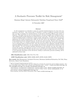
can be solved exactly. The following charts plot a number of simulated sample paths using the above
equation and the mean plus/minus one standard deviation and the ﬁrst and 99th percentiles over time.
The mean of the asset price grows exponentially with time.

350 300

300
250

250
200
Spot Price

Spot Price
200

150
150

100
100

50 50
0 100 200 300 400 500 600 0 100 200 300 400 500
Time in days Time in days

Figure 1: GBM Sample Paths and Distribution Statistics

The following Matlab function simulates sample paths of the GBM using equation (7), which was
vectorised in Matlab.

Code 1 M AT LAB Code to simulate GBM Sample Paths.
function S = G B M _ s i m u l a t i o n( N_Sim ,T , dt , mu , sigma , S0 )

mean =( mu -0.5* sigma ^2)* dt ;
S = S0 * ones ( N_Sim , T +1);

BM = sigma * sqrt ( dt )* normrnd (0 ,1 , N_Sim , T );
S (: ,2: end )= S0 * exp ( cumsum ( mean + BM ,2));

end

2.2 Parameter Estimation
This section describes how the GBM can be used as an attempt to model the random behaviour of the
FTSE100 stock index, the log of which is plotted in the left chart of Figure 2.

The second chart, on the right of Figure 2, plots the quantiles of the log return distribution against
the quantiles of the standard normal distribution. This QQ-plot allows one to compare distributions
and to check the assumption of normality. The quantiles of the historical distribution are plotted on the
Y-axis and the quantiles of the chosen modeling distribution on the X-axis. If the comparison distribution
provides a good ﬁt to the historical returns, then the QQ-plot approximates a straight line. In the case


QQ Plot of Sample Data versus Standard Normal
10
8
8
7
6
6

Quantiles of Input Sample
4
log of FTSE 100 Index

5 2

4 0

−2
3
−4
2
−6

1
−8

0 −10
1940 1946 1953 1959 1965 1971 1978 1984 1990 1996 2003 −4 −3 −2 −1 0 1 2 3 4
Standard Normal Quantiles

Figure 2: Historical FTSE100 Index and QQ Plot FTSE 100

of the FTSE100 log returns, the QQ-plot show that the historical quantiles in the tail of the distribution
are significantly larger compared to the normal distribution. This is in line with the general observation
about the presence of fat tails in the return distribution of financial asset prices. Therefore the GBM
at best provides only a rough approximation for the FTSE100. The next sections will outline some
extensions of the GBM that provide a better fit to the historical distribution.
Another important property of the GBM is the independence of returns. Therefore, to ensure the
GBM is appropriate for modelling the asset price in a financial time series one has to check that the
returns of the observed data are truly independent. The assumption of independence in statistical terms
means that there is no autocorrelation present in historical returns. A common test for autocorrelation
(typically on returns of a given asset) in a time series sample x1 , x2 , . . . , xn realised from a random process
X(ti ) is to plot the autocorrelation function of the lag k, defined as:
n−k
1
ACF(k) = (xi − m)(xi+k − m), k = 1, 2, . . .
ˆ ˆ (8)
(n − k)ˆ
v i=1
where m and v are the sample mean and variance of the series, respectively. Often, besides the ACF,
ˆ ˆ
one also considers the Partial Auto-Correlation function (PACF). Without fully defining PACF, roughly
speaking one may say that while ACF(k) gives an estimate of the correlation between X(ti ) and X(ti+k ),
PACF(k) informs on the correlation between X(ti ) and X(ti+k ) that is not accounted for by the shorter
lags from 1 to k − 1, or more precisely it is a sort of sample estimate of:

Corr(X(ti ) − Xii+1,...,i+k−1 , X(ti+k ) − Xi+k
¯ ¯ i+1,...,i+k−1 )

where Xii+1,...,i+k−1 and Xi+k
¯ ¯ i+1,...,i+k−1 are the best estimates (regressions in a linear context) of X(ti )
and X(ti+k ) given X(ti+1 ), . . . , X(ti+k−1 ). PACF also gives an estimate of the lag in an autoregressive
process.
ACF and PACF for the FTSE 100 equity index returns are shown in the charts in Figure 3. For the
FTSE100 one does not observe any significant lags in the historical return time series, which means the
independence assumption is acceptable in this example.
Maximum Likelihood Estimation

Having tested the properties of independence as well as normality for the underlying historical data
one can now proceed to calibrate the parameter set Θ = (µ, σ) for the GBM based on the historical
returns. To find Θ that yields the best fit to the historical dataset the method of maximum likelihood
estimation is used (MLE).

MLE can be used for both continuous and discrete random variables. The basic concept of MLE, as
suggested by the name, is to find the parameter estimates Θ for the assumed probability density function


Sample Autocorrelation Function (ACF) Sample Partial Autocorrelation Function

0.8 0.8

Sample Partial Autocorrelations
Sample Autocorrelation

0.6 0.6

0.4 0.4

0.2 0.2

0 0

−0.2 −0.2
0 5 10 15 20 0 5 10 15 20
Lag Lag

Figure 3: Autocorrelation and Partial Autocorrelation Function for FTSE 100

fΘ (continuous case) or probability mass function (discrete case) that will maximise the likelihood or
probability of having observed the given data sample x1 , x2 , x3 , ..., xn for the random vector X1 , ..., Xn .
In other terms, the observed sample x1 , x2 , x3 , ..., xn is used inside fX1 ,X2 ,...,Xn ;Θ , so that the only variable
in f is Θ, and the resulting function is maximised in Θ. The likelihood (or probability) of observing a
particular data sample, i.e. the likelihood function, will be denoted by L(Θ).
In general, for stochastic processes, the Markov property is sufficient to be able to write the likelihood
along a time series of observations as a product of transition likelihoods on single time steps between
two adjacent instants. The key idea there is to notice that for a Markov process xt , one can write, again
denoting f the probability density of the vector random sample:
L(Θ) = fX(t0 ),X(t1 ),...,X(tn );Θ = fX(tn )|X(tn−1 );Θ · fX(tn−1 )|X(tn−2 );Θ · · · fX(t1 )|X(t0 );Θ · fX(t0 );Θ (9)
In the more extreme cases where the observations in the data series are iid, the problem is consid-
erably simplified, since fX(ti )|X(ti−1 );Θ = fX(ti );Θ and the likelihood function becomes the product of
the probability density of each data point in the sample without any conditioning. In the GBM case,
this happens if the maximum likelihood estimation is done on log-returns rather than on the levels. By
defining the X as
X(ti ) := log S(ti ) − log S(ti−1 ), (10)
one sees that they are already independent so that one does not need to use explicitly the above decom-
position (9) through transitions. For general Markov processes different from GBM, or if one had worked
at level space S(ti ) rather than in return space X(ti ), this can be necessary though: see, for example,
the Vasicek example later on.
The likelihood function for iid variables is in general:
n
L(Θ) = fΘ (x1 , x2 , x3 , ..., xn ) = fΘ (xi ) (11)
i=1

ˆ
The MLE estimate Θ is found by maximising the likelihood function. Since the product of density
values could become very small, which would cause numerical problems with handling such numbers,
the likelihood function is usually converted6 to the log likelihood L∗ = log L.7 For the iid case the
log-likelihood reads:
n
L∗ (Θ) = log fΘ (xi ) (12)
i=1
6 This is allowed, since maxima are not affected by monotone transformations.
7 The reader has to be careful not to confuse the log taken to move from levels S to returns X with the log used to move
from the likelihood to the log-likelihood. The two are not directly related, in that one takes the log-likelihood in general
even in situations when there are no log-returns but just general processes.


The maximum of the log likelihood usually has to be found numerically using an optimisation algo-
rithm8 . In the case of the GBM, the log-returns increments form normal iid random variables, each with
a well known density fΘ (x) = f (x; m, v), determined by mean and variance. Based on Equation (3) (with
u = ti+1 and t = ti ) the parameters are computed as follows:

1
m = µ − σ 2 ∆t
ˆ v = σ 2 ∆t (13)
2
The estimates for the GBM parameters are deduced from the estimates of m and v. In the case of
the GBM, the MLE method provides closed form expressions for m and v through MLE of Gaussian iid
samples9 . This is done by differentiating the Gaussian density function with respect to each parameter and
setting the resulting derivative equal to zero. This leads to following well known closed form expressions
for the sample mean and variance10 of the log returns samples xi for Xi = log S(ti ) − log S(ti−1 )
n n
m=
ˆ xi /n v=
ˆ (xi − m)2 /n.
ˆ (14)
i=1 i=1

Similarly one can find the maximum likelihood estimates for both parameters simultaneously using
the following numerical search algorithm.

Code 2 M AT LAB MLE Function for iid Normal Distribution.
function [ mu sigma ] = G B M _ c a l i b r a t i o n(S , dt , params )
Ret = p r i c e 2 r e t( S );
n = length ( Ret );
options = optimset ( ’ M a x F u n E v a l s’ , 100000 , ’ MaxIter ’ , 100 000);
f m i n s e a r c h( @normalLL , params , options );
function mll = normalLL ( params )
mu = params (1); sigma = abs ( params (2));
ll = n * log (1/ sqrt (2* pi * dt )/ sigma )+ sum ( -( Ret - mu * dt ).^2/2/( dt * sigma ^2));
mll = - ll ;
end
end

An important remark is in order for this important example: given that xi = log s(ti ) − log s(ti−1 ),
where s is the observed sample time series for geometric brownian motion S, m is expressed as:
ˆ
n
log(s(tn )) − log(s(t0 ))
m=
ˆ xi /n = (15)
i=1
n
The only relevant information used on the whole S sample are its initial and final points. All of the
remaining sample, possibly consisting of hundreds of observations, is useless.11

This is linked to the fact that drift estimation for random processes like GBM is extremely difficult.
In a way, if one could really estimate the drift one would know locally the direction of the market in
the future, which is effectively one of the most difficult problems. The impossibility of estimating this
quantity with precision is what keeps the market alive. This is also one of the reasons for the success of
risk neutral valuation: in risk neutral pricing one is allowed to replace this very difficult drift with the
risk free rate.
8 For example, Excel Solver or fminsearch in MatLab, although for potentially multimodal likelihoods, such as possibly

the jump diffusion cases further on, one may have to preprocess the optimisation through a coarse grid global method such
as genetic algorithms or simulated annealing, so as to avoid getting stuck in a local minima given by a lower mode.
9 Hogg and Craig, Introduction to Mathematical Statistics., fourth edition, p. 205, example 4.
10 Note that the estimator for the variance is biased, since E(ˆ) = v(n − 1)/n. The bias can be corrected by multiplying
v
the estimator by n/(n − 1). However, for large data samples the difference is very small.
11 Jacod, in Statistics of Diffusion Processes: Some Elements, CNR-IAMI 94.17, p. 2, in case v is known, shows that the

drift estimation can be statistically consistent, converging in probability to the true drift value, only if the number of points
times the time step tends to infinity. This confirms that increasing the observations between two given fixed instants is
useless; the only helpful limit would be letting the final time of the sample go to infinity, or let the number of observations
increase while keeping a fixed time step


The drift estimation will improve considerably for mean reverting processes, as shown in the next
sections.

Confidence Levels for Parameter Estimates
For most applications it is important to know the uncertainty around the parameter estimates obtained
from historical data, which is statistically expressed by confidence levels. Generally, the shorter the
historical data sample, the larger the uncertainty as expressed by wider confidence levels.
For the GBM one can derive closed form expressions for the Confidence Interval (CI) of the mean
and standard deviation of returns, using the Gaussian law of independent return increments and the fact
that the sum of independent Gaussians is still Gaussian, with the mean given by the sum of the means
and the variance given by the sum of variances. Let Cn = X1 + X2 + X3 + ... + Xn , then one knows that
Cn ∼ N (nm, nv) 12 . One then has:

Cn − nm Cn /n − m
P √ √ z =P √ √ z = Φ(z) (16)
v n v/ n
where Φ() denotes the cumulative standard normal distribution. Cn /n, however, is the MLE estimate
for the sample mean m. Therefore the 95th confidence level for the sample mean is given by:
√ √
Cn v Cn v
− 1.96 √ m + 1.96 √ (17)
n n n n
This shows that as n increases the CI tightens, which means the uncertainty around the parameter
estimates declines.

Since a standard Gaussian squared is a chi-squared, and the sum of n independent chi-squared is a
chi-squared with n degrees of freedom, this gives:
n 2
(xi − m)
ˆ n
P √ z =P v
ˆ z = χ2 (z),
n (18)
i=1
v v
hence under the assumption that the returns are normal one finds the following confidence interval
for the sample variance:
n n
χvˆ v χvˆ (19)
qU qL
χ χ
where qL , qU are the quantiles of the chi-squared distribution with n degrees of freedom corresponding
to the desired confidence level.
In the absence of these explicit relationships one can also derive the distribution of each of the pa-
rameters numerically, by simulating the sample parameters as follows. After the parameters have been
estimated (either through MLE or with the best fit to the chosen model, call these the ”first parame-
ters”), simulate a sample path of length equal to the historical sample with those parameters. For this
sample path one then estimates the best fit parameters as if the historical sample were the simulated
one, and obtains a sample of the parameters. Then again, simulating from the first parameters, one
goes through this procedure and obtains another sample of the parameters. By iterating one builds a
random distribution of each parameter, all starting from the first parameters. An implementation of the
simulated parameter distributions is provided in the next Matlab function.

The charts in Figure 4 plot the simulated distribution for the sample mean and sample variance
against the normal and Chi-squared distribution given by the theory and the Gaussian distribution. In
both cases the simulated distributions are very close to their theoretical limits. The confidence levels
and distributions of individual estimated parameters only tell part of the story. For example, in value-
at-risk calculations, one would be interested in finding a particular percentile of the asset distribution.
In expected shortfall calculations, one would be interested in computing the expectation of the asset
12 Even without the assumption of Gaussian log returns increments, but knowing only that log returns increments are

iid, one can reach a similar Gaussian limit for Cn , but only asymptotically in n, thanks to the central limit theorem.


Code 3 M AT LAB Simulating distribution for Sample mean and variance.
% load ’C : Research QS CVO T e c h n i c a l Paper Report Chapte r1 f t s e 1 0 0 m o n t h l y 1 9 4 0. mat ’
load ’ f t s e 1 0 0 m o n t h l y 1 9 4 0. mat ’
S = f t s e 1 0 0 m o n t h l y 1 9 4 0 d a t a;
ret = log ( S (2: end ,2)./ S (1: end -1 ,2));
n = length ( ret )

m = sum ( ret )/ n
v = sqrt ( sum (( ret - m ).^2)/ n )

SimR = normrnd (m ,v ,10000 ,n );

m_dist = sum ( SimR ,2)/ n ;
m_tmp = repmat ( m_dist ,1 ,799);
v_dist = sum (( SimR - m_tmp ).^2 ,2)/ n ;

dt =1/12;
s i g m a _ d i s t= sqrt ( v_dist / dt );
mu_dist = m_dist / dt +0.5* s i g m a _ d i s t .^2;

S0 =100;
pct_dist = S0 * logninv (0.99 , sigma_dist , mu_dist );

0.035 0.035

0.03 0.03

0.025 0.025
Frequency

Frequency

0.02 0.02

0.015 0.015

0.01 0.01

0.005 0.005

0 0
0.05 0.1 0.15 0.2 600 650 700 750 800 850 900 950 1000
GBM Parameter mu Normalised Sample Variance

Figure 4: Distribution of Sample Mean and Variance

conditional on exceeding such percentile. In the case of the GBM, one knows the marginal distribution
of the asset price to be log normal and one can compute percentiles analytically for a given parameter
set. The MATLAB code 2.2, which computes the parameter distributions, also simulates the distribution
for the 99th percentile of the asset price after three years when re-sampling from simulation according to
the first estimated parameters. The histogram is plotted in Figure 5.

2.3 Characteristic and Moment Generating Functions
Let X be a random variable, either discrete with probability pX (first case) or continuous with density
fX (second case). The k − th moment mk (X) is defined as:
k
mk (X) = E(X k ) = x x pX (x)
∞
−∞
xk fX (x)dx.

Moments are not guaranteed to exist, for example the Cauchy distribution does not even admit the first
moment (mean). The moment generating function MX (t) of a random variable X is defined, under some
technical conditions for existence, as:
tx
x e pX (x)
M (t) = E(etX ) = ∞
−∞
etx fX (x)dx


0.035

0.03

0.025

Frequency
0.02

0.015

0.01

0.005

0
130 140 150 160 170 180 190 200
99th Percentile with S0=100 over a three year period

Figure 5: Distribution for 99th Percentile of FTSE100 over a three year Period

and can be seen to be the exponential generating function of its sequence of moments:
∞
mk (X) k
MX (t) = t . (20)
k!
k=0

The moment generating function (MGF) owes its name to the fact that from its knowledge one may back
out all moments of the distribution. Indeed, one sees easily that by differentiating j times the MGF and
computing it in 0 one obtains the j-th moment:

dj
MX (t)|t=0 = mj (X). (21)
dtj
A better and more general definition is that of characteristic function, defined as:

φX (t) = E(eitX ),

where i is the unit imaginary number from complex numbers theory. The characteristic function exists for
every possible density, even for the Cauchy distribution, whereas the moment generating function does not
exist for some random variables, notably some with infinite moments. If moments exist, one can derive
them also from the characteristic function through differentiation. Basically, the characteristic function
forces one to bring complex numbers into the picture but brings in considerable advantages. Finally, it
is worth mentioning that the moment generating function can be seen as the Laplace transform of the
probability density, whereas the characteristic function is the Fourier transform.

2.4 Properties of Moment Generating and Characteristic Functions
If two random variables, X and Y , have the same moment generating function M (t), then X and Y have
the same probability distribution. The same holds, more generally, for the characteristic function.
If X and Y are independent random variables and W = X + Y , then the moment generating function
of W is the product of the moment generating functions of X and Y :

MX+Y (t) = E(et(X+Y ) ) = E(etX etY ) = E(etX )E(etY ) = MX (t)MY (t).

The same property holds for the characteristic function. This is a very powerful property since the sum
of independent returns or shocks is common in modelling. Finding the density of a sum of independent
random variables can be difficult, resulting in a convolution, whereas in moment or characteristic function
space it is simply a multiplication. This is why typically one moves in moment generating space, computes
a simple multiplication and then goes back to density space rather than working directly in density space
through convolution.


As an example, if X and Y are two independent random variables and X is normal with mean µ1 and
2 2
variance σ1 and Y is normal with mean µ2 and variance σ2 , then one knows that W = X + Y is normal
2 2
with mean µ1 + µ2 and variance σ1 + σ2 . In fact, the moment generating function of a normal random
variable Z ∼ N (µ, σ 2 ) is given by:
σ2 2
MZ (t) = eµt+ 2 t

Hence 2 2
σ1 2 σ2 2
MX (t) = eµ1 t+ 2 t and MY (t) = eµ2 t+ 2 t

From this 2 2 2 2
σ1 2 σ2 2 (σ1 +σ2 ) 2
MW (t) = MX (t)MY (t) = eµ1 t+ 2 t eµ2 t+ 2 t = e(µ1 +µ2 )t+ 2 t

one obtains the moment generating function of a normal random variable with mean (µ1 + µ2 ) and
2 2
variance (σ1 + σ2 ), as expected.

3 Fat Tails: GARCH Models
GARCH13 models were first introduced by Bollerslev (1986). The assumption underlying a GARCH
model is that volatility changes with time and with the past information. In contrast, the GBM model
introduced in the previous section assumes that volatility (σ) is constant. GBM could have been easily
generalised to a time dependent but fully deterministic volatility, not depending on the state of the
process at any time. GARCH instead allows the volatility to depend on the evolution of the process. In
particular the GARCH(1,1) model, introduced by Bollerslev, assumes that the conditional variance (i.e.
conditional on information available up to time ti ) is given by a linear combination of the past variance
σ(ti−1 )2 and squared values of past returns.

∆S(ti )
= µ∆ti + σ(ti )∆W (ti )
S(ti )
σ(ti )2 = ω¯ 2 + ασ(ti−1 )2 + βǫ(ti−1 )2
σ
2
ǫ(ti )2 = (σ(ti )∆W (ti )) (22)

where ∆S(ti ) = S(ti+1 ) − S(ti ) and the first equation is just the discrete time counterpart of Equation
(1).
If one had just written the discrete time version of GBM, σ(ti ) would just be a known function of time
and one would stop with the first equation above. But in this case, in the above GARCH model σ(t)2 is
assumed itself to be a stochastic process, although one depending only on past information. Indeed, for
example
σ(t2 )2 = ω¯ 2 + βǫ(t1 )2 + αω¯ 2 + α2 σ(t0 )2
σ σ
so that σ(t2 ) depends on the random variable ǫ(t1 )2 . Clearly conditional on the information at the
previous time t1 the volatility is no longer random, but unconditionally it is, contrary to the GBM
volatility.
In GARCH the variance is an autoregressive process around a long-term average variance rate σ 2 . ¯
The GARCH(1,1) model assumes one lag period in the variance. Interestingly, with ω = 0 and β = 1 − α
one recovers the exponentially weighted moving average model, which unlike the equally weighted MLE
estimator in the previous section, puts more weight on the recent observations. The GARCH(1,1) model
can be generalised to a GARCH(p, q) model with p lag terms in the variance and q terms in the squared
returns. The GARCH parameters can be estimated by ordinary least squares regression or by maximum
likelihood estimation, subject to the constraint ω + α + β = 1, a constraint summarising of the fact that
the variance at each instant is a weighted sum where the weights add up to one.
As a result of the time varying state-dependent volatility, the unconditional distribution of returns is
non-Gaussian and exhibits so called “fat” tails. Fat tail distributions allow the realizations of the random
variables having those distributions to assume values that are more extreme than in the normal/Gaussian
13 Generalised Autoregressive Conditional Heteroscedasticity


0.1 8
Historical
0.09 NGARCH Sim
6
Normal
0.08
4
0.07
2
0.06

Y Quantiles
Frequency

0.05 0

0.04
−2
0.03
−4
0.02
−6
0.01

0 −8
−10 −5 0 5 10 −8 −6 −4 −2 0 2 4 6 8
Historical vs Simulated Return Distribution X Quantiles

Figure 6: Historical FTSE100 Return Distribution vs. NGARCH Return Distribution

case, and are therefore more suited to model risks of large movements than the Gaussian. Therefore,
returns in GARCH will tend to be “riskier” than the Gaussian returns of GBM.
GARCH is not the only approach to account for fat tails, and this report will introduce other ap-
proaches to fat tails later on.
The particular structure of the GARCH model allows for volatility clustering (autocorrelation in the
volatility), which means a period of high volatility will be followed by high volatility and conversely
a period of low volatility will be followed by low volatility. This is an often observed characteristic
of financial data. For example, Figure 8 shows the monthly volatility of the FTSE100 index and the
corresponding autocorrelation function, which confirms the presence of autocorrelation in the volatility.
A long line of research followed the seminal work of Bollerslev leading to customisations and general-
isations including exponential GARCH (EGARCH) models, threshold GARCH (TGARCH) models and
non-linear GARCH (NGARCH) models among others. In particular, the NGARCH model introduced by
Engle and Ng (1993) is an interesting extension of the GARCH(1,1) model, since it allows for asymmetric
behaviour in the volatility such that “good news” or positive returns yield subsequently lower volatility,
while “bad news” or negative returns yields a subsequent increase in volatility. The NGARCH is specified
as follows:

∆S(ti )
= µ∆ti + σ(ti )∆W (ti )
S(ti )
2
σ(ti )2 = ω + ασ(ti−1 )2 + β (ǫ(ti−1 ) − γσ(ti−1 ))
ǫ(ti )2 = (σ(ti )∆W (ti ))2 (23)

NGARCH parameters ω, α, and β are positive and α, β, and γ are subject to the stationarity
constraint α + β(1 + γ 2 ) < 1.
Compared to the GARCH(1,1), this model contains an additional parameter γ, which is an adjustment
to the return innovations. Gamma equal to zero leads to the symmetric GARCH(1,1) model, in which
positive and negative ǫ(ti−1 ) have the same effect on the conditional variance. In the NGARCH γ is
positive, thus reducing the impact of good news (ǫ(ti−1 ) > 0) and increasing the impact of bad news
(ǫ(ti−1 ) < 0) on the variance.
MATLAB Routine 4 extends Routine 1 by simulating the GBM with the NGARCH volatility struc-
ture. Notice that there is only one loop in the simulation routine, which is the time loop. Since the
GARCH model is path dependent it is no longer possible to vectorise the simulation over the time step.
For illustration purpose, this model is calibrated to the historic asset returns of the FTSE100 index. In
order to estimate the parameters for the NGARCH geometric Brownian motion the maximum-likelihood
method introduced in the previous section is used.


Market News

2

News level
0

−2

100 200 300 400 500 600 700 800 900 1000
4 years of daily simulation
GBM Log returns Volatility with GARCH effects
0.1
Log returns Volatility

0.08

0.06

0.04

0.02

0
100 200 300 400 500 600 700 800 900 1000
GBM Log returns Volatility with N−GARCH effects
0.1
Log returns Volatility

0.08

0.06

0.04

0.02

0
100 200 300 400 500 600 700 800 900 1000

GBM Log returns

0.1
Log returns

0.05

0

−0.05
100 200 300 400 500 600 700 800 900 1000
GBM Log returns with GARCH effects

0.1
Log returns

0.05

0

−0.05
100 200 300 400 500 600 700 800 900 1000
GBM Log returns with N−GARCH effects

0.1
Log returns

0.05

0

−0.05
100 200 300 400 500 600 700 800 900 1000

Figure 7: NGARCH News Eﬀect vs GARCH News Eﬀect

Although the variance is changing over time and is state dependent and hence stochastic conditional on
information at the initial time, it is locally deterministic, which means that conditional on the information
at ti−1 the variance is known and constant in the next step between time ti−1 and ti . In other words,


Sample Autocorrelation Function (ACF)
4

3.5
0.8

3

Sample Autocorrelation
0.6
Monthly volatily in %

2.5

2 0.4

1.5
0.2

1

0
0.5

0 −0.2
1940 1946 1953 1959 1965 1971 1978 1984 1990 1996 2003 0 5 10 15 20
Lag

Figure 8: Monthly Volatility of the FTSE100 and Autocorrelation Function

Code 4 M AT LAB Code to Simulate GBM with NGARCH vol.
function S = N G A R C H _ s i m u l a t i o n( N_Sim ,T , params , S0 )
mu_ = params (1); omega_ = params (2); alpha_ = params (3); bet a_ = params (4); gamma_ = params (5);
S = S0 * ones ( N_Sim , T );
v0 = omega_ /(1 - alpha_ - beta_ );
v = v0 * ones ( N_Sim ,1);
BM = normrnd (0 ,1 , N_Sim , T );
for i =2: T
sigma_ = sqrt ( v );
mean =( mu_ -0.5* sigma_ .^2);
S (: , i )= S (: , i -1).* exp ( mean + sigma_ .* BM (: , i ));
v = omega_ + alpha_ * v + beta_ *( sqrt ( v ).* BM (: , i ) - gamma_ * sqrt ( v )).^2;
end
end

the variance in the GARCH models is locally constant. Therefore, conditional on the variance at ti−1
the density of the process at the next instant is still normal14 . Moreover, the conditional returns are still
independent. The log-likelihood function for the sample x1 , ..., xi , ..., xn of:
∆S(ti )
Xi =
S(ti )
is given by:
n
L∗ (Θ) = log fΘ (xi ; xi−1 ) (24)
i=1

2 1 (xi − µ)2
fΘ (xi ; xi−1 ) = fN (xi ; µ, σi ) = exp − 2 (25)
2
2πσi 2σi
1
L∗ (Θ) = constant + − log(σi ) − (xi − µ)2 /σi
2 2
(26)
2
where fΘ is the density function of the normal distribution. Note the appearance of xi−1 in the func-
tion, which indicates that normal density is only locally applicable between successive returns, as noticed
previously. The parameter set for the NGARCH GBM includes ﬁve parameters, Θ = (µ, ω, α, β, γ). Due
to the time changing state dependent variance one no longer ﬁnds explicit solutions for the individual
parameters and has to use a numerical scheme to maximise the likelihood function through a solver. To
do so one only needs to maximise the term in brackets in (26), since the constant and the factor do not
depend on the parameters.
14 Note that the unconditional density of the NGARCH GBM is no longer normal, but an unknown heavy tailed distri-

bution.


Code 5 M AT LAB Code to Estimate Parameters for GBM NGARCH.
function [ mu_ omega_ alpha_ beta_ gamma_ ]= N G _ c a l i b r a t i o n( data , pa rams )
returns = p r i c e 2 r e t( data );
r e t u r n s L e n g t h= length ( returns );
f m i n s e a r c h( @NG_JGBM_LL , params , options );
function mll = N G _ J G B M _ L L( params )
mu_ = params (1); omega_ = abs ( params (2)); alpha_ = abs ( params (3));
beta_ = abs ( params (4)); gamma_ = params (5);
denum = 1 - alpha_ - beta_ *(1+ gamma_ ^2);
if denum < 0; mll = intmax ; return ; end % Variance s t a t i o n a r i t y test
var_t = omega_ / denum ;
innov = returns (1) - mu_ ;
L o g L i k e l i h o o d = log ( exp ( - innov ^2/ var_t /2)/ sqrt ( pi *2* var_t ));
for time =2: r e t u r n s L e n g t h
var_t = omega_ + alpha_ * var_t + beta_ *( innov - gamma_ * sqrt ( var_t ))^2;
if var_t <0; mll = intmax ; return ; end ;
innov = returns ( time ) - mu_ ;
L o g L i k e l i h o o d = L o g L i k e l i h o o d + log ( exp ( - innov ^2/ var_t /2)/ sqrt ( pi *2* var_t ));
end
mll = - L o g L i k e l i h o o d;
end
end

Having estimated the best fit parameters one can verify the fit of the NGARCH model for the FTSE100
monthly returns using the QQ-plot. A large number of monthly returns using Routine 5 is first simulated.
The QQ plot of the simulated returns against the historical returns shows that the GARCH model
does a significantly better job when compared to the constant volatility model of the previous section.
The quantiles of the simulated NGARCH distribution are much more aligned with the quantiles of the
historical return distribution than was the case for the plain normal distribution (compare QQ-plots in
Figures 2 and 6).

4 Fat Tails: Jump Diffusion Models
Compared with the normal distribution of the returns in the GBM model, the log-returns of a GBM model
with jumps are often leptokurtotic15 . This section discusses the implementation of a jump-diffusion model
with compound Poisson jumps. In this model, a standard time homogeneous Poisson process dictates
the arrival of jumps, and the jump sizes are random variables with some preferred distribution (typically
Gaussian, exponential or multinomial). Merton (1976) applied this model to option pricing for stocks
that can be subject to idiosyncratic shocks, modelled through jumps. The model SDE can be written as:

dS(t) = µS(t)dt + σS(t)dW (t) + S(t)dJt (27)
where again Wt is a univariate Wiener process and Jt is the univariate jump process defined by:
NT
JT = (Yj − 1), or dJ(t) = (YN (t) − 1)dN (t), (28)
j=1

where (NT )T 0 follows a homogeneous Poisson process with intensity λ, and is thus distributed like a
Poisson distribution with parameter λT . The Poisson distribution is a discrete probability distribution
that expresses the probability of a number of events occurring in a fixed period of time. Since the Poisson
distribution is the limiting distribution of a binomial distribution where the number of repetitions of the
Bernoulli experiment n tends to infinity, each experiment with probability of success λ/n, it is usually
adopted to model the occurrence of rare events. For a Poisson distribution with parameter λT , the
Poisson probability mass function is:

exp(−λT )(λT )x
fP (x, λT ) = , x = 0, 1, 2, . . .
x!
15 Fat-tailed distribution.


(recall that by convention 0! = 1). The Poisson process (NT )T 0 is counting the number of arrivals in
2
[1, T ], and Yj is the size of the j-th jump. The Y are i.i.d log-normal variables (Yj ∼ exp N µY , σY )
that are also independent from the Brownian motion W and the basic Poisson process N .

Also in the jump diffusion case, and for comparison with (2), it can be useful to write the equation
for the logarithm of S, which in this case reads
1
d log S(t) = µ − σ 2 dt + σdW (t) + log(YN (t) )dN (t) or, equivalently (29)
2
1
d log S(t) = µ + λµY − σ 2 dt + σdW (t) + [log(YN (t) )dN (t) − µY λdt]
2
where now both the jump (between square brackets) and diffusion shocks have zero mean, as is shown
right below. Here too it is convenient to do MLE estimation in log-returns space, so that here too one
defines X(ti )’s according to (10).
The solution of the SDE for the levels S is given easily by integrating the log equation:
N (T )
σ2
S(T ) = S(0) exp µ− T + σW (T ) Yj (30)
2 j=1

Code 6 M AT LAB Code to Simulate GBM with Jumps.
function S = J G B M _ s i m u l a t i o n( N_Sim ,T , dt , params , S0 )
mu_star = params (1); sigma_ = params (2); lambda_ = params (3 );
mu_y_ = params (4); sigma_y_ = params (5);
M_simul = zeros ( N_Sim , T );
for t =1: T
jumpnb = poissrnd ( lambda_ * dt , N_Sim ,1);
jump = normrnd ( mu_y_ *( jumpnb - lambda_ * dt ) , sqrt ( jumpnb )* sigma_y_ );
M_simul (: , t ) = mu_star * dt + sigma_ * sqrt ( dt )* randn ( N_Sim ,1) + jump ;
end
S = r e t 2 p r i c e( M_simul ’ , S0 ) ’;
end

The discretisation of the Equation (30) for the given time step ∆t is:
nt
σ2 √
S(t) = S(t − ∆t) exp µ− ∆t + σ ∆tεt Yj (31)
2 j=1

where ε ∼ N (0, 1) and nt = Nt − Nt−∆t counts the jumps between time t − ∆t and t. When rewriting
this equation for the log returns
X(t) := ∆ log(S(t)) = log(S(t)) − log(S(t − ∆t)) we find:
√
X(t) = ∆ log(S(t)) = µ∗ ∆t + σ ∆t εt + ∆Jt
∗
(32)

where the jumps ∆Jt in the time interval ∆t and the drift µ∗ are defined as:
∗

nt
∗ 1
∆Jt = log(Yj ) − λ ∆t µY , µ∗ = µ + λµY − σ 2 (33)
j=1
2
∗
so that the jumps ∆Jt have zero mean. Since the calibration and simulation are done in a discrete time
framework, we use the fact that for the Poisson process with rate λ, the number of jump events occurring
in the fixed small time interval ∆t has the expectation of λ∆t. Compute
    
nt nt
∗
E(∆Jt ) = E log Yj  − λ ∆t µY = E E  log Yj |nt  − λ ∆t µY
j=1 j=1

= E (nt µY ) − λ ∆t µY = 0


Jumps
0.06

0.05

Jumps log return level 0.04

0.03

0.02

0.01

0

−0.01
0 50 100 150 200 250
1 year of daily simulation

GBM (black line) and GBM with Jumps (green line)
0.05

0.048

0.046
S(t)

0.044

0.042

0.04

0.038
0 50 100 150 200 250
1 year of daily simulation

GBM histogram GBM with Jumps histogram
0.014 0.014

0.012 0.012

0.01 0.01
Frequency

Frequency

0.008 0.008

0.006 0.006

0.004 0.004

0.002 0.002

0 0
−0.06 −0.04 −0.02 0 0.02 0.04 0.06 −0.06 −0.04 −0.02 0 0.02 0.04 0.06
Simulated daily log return Simulated daily log return

Figure 9: The Eﬀect of the Jumps on the Simulated GBM path and on the Density Probability of the
Log Returns. µ∗ = 0, σ = 0.15, λ = 10, µY = 0.03, σY = 0.001

The simulation of this model is best done by using Equation (32).
∗
Conditional on the jumps occurrence nt , the jump disturbance ∆Jt is normally distributed
∗ 2
∆Jt |nt ∼ N (nt − λ∆t)µY , nt σY .

Thus the conditional distribution of X(t) = ∆ log(S(t)) is also normal and the ﬁrst two conditional
moments are:

E(∆ log(S(t))|nt ) = µ∗ ∆t + (nt − λ ∆t)µY = µ − σ 2 /2 ∆t + nt µY , (34)
2 2
Var(∆ log(S(t))|nt ) = σ ∆t + nt σY (35)

The probability density function is the sum of the conditional probabilities density weighted by the
probability of the conditioning variable: the number of jumps. Then the calibration of the model param-
eters can be done using the MLE on log-returns X conditioning on the jumps.


Code 7 M AT LAB Code to Calibrate GBM with Jumps.
function [ mu_star sigma_ lambda_ mu_y_ sigma_y_ ] = J G B M _ c a l i b r a t i o n( data , dt , params )
returns = p r i c e 2 r e t( data );
d a t a L e n g t h= length ( data );
params = f m i n s e a r c h( @FT_JGBM_LL , params , options );
mu_star = params (1); sigma_ = abs ( params (2)); lambda_ = abs ( params (3));
mu_y_ = params (4); sigma_y_ = abs ( params (5));

function mll = F T _ J G B M _ L L( params )
mu_ = params (1); sigma_ = abs ( params (2)); lambda_ = abs ( params (3));
mu_y_ = params (4); sigma_y_ = abs ( params (5));
M a x _ j u m p s = 5;
f a c t o r i e l = f a c t o r i a l(0: M a x _ j u m p s);
L o g L i k e l i h o o d = 0;
for time =1: d a t a L e n g t h
P r o b D e n s i t y = 0;
for jumps =0: Max_jumps -1
jumpProb = exp ( - lambda_ * dt )*( lambda_ * dt )^ jumps / f a c t o r i e l( jumps +1) ;
condVol = dt * sigma_ ^2+ jumps * sigma_y_ ^2;
condMean = mu_ * dt + mu_y_ *( jumps - lambda_ * dt );
c o n d T o J u m p s = exp ( -( data ( time ) - condMean )^2/ condVol /2)/ sqrt ( pi *2* condVol );
P r o b D e n s i t y = P r o b D e n s i t y + jumpProb * c o n d T o J u m p s;
end
L o g L i k e l i h o o d = L o g L i k e l i h o o d + log ( P r o b D e n s i t y);
end
mll = - L o g L i k e l i h o o d;

end
end

argmax L∗ = log(L) (36)
µ∗ ,µY ,λ>0,σ>0,σY >0

The log-likelihood function for the returns X(t) at observed times t = t1 , . . . , tn with values x1 , . . . , xn ,
with ∆t = ti − ti−1 , is then given by:

n
∗
L (Θ) = log f (xi ; µ, µY , λ, σ, σY ) (37)
i=1
+∞
f (xi ; µ, µY , λ, σ, σY ) = P (nt = j)fN xi ; µ − σ 2 /2 ∆t + jµY , σ 2 ∆t + jσY
2
(38)
j=0

This is an infinite mixture of Gaussian random variables, each weighted by a Poisson probability
P (nt = j) = fP (j; λ∆t). Notice that if ∆t is small, typically the Poisson process jumps at most once. In
that case, the above expression simplifies in

f (xi ; µ, µY , λ, σ, σY ) = (1 − λ∆t)fN xi ; µ − σ 2 /2 ∆t, σ 2 ∆t
+ λ ∆t fN xi ; µ − σ 2 /2 ∆t + µY , σ 2 ∆t + σY
2

i.e. a mixture of two Gaussian random variables weighted by the probability of zero or one jump in ∆t.
The model parameters are estimated by MLE for FTSE100 on monthly returns and then different
paths are simulated. The goodness to fit is seen by showing the QQ-plot of the simulated monthly log
returns against the historical FTSE100 monthly returns in Fig. 10. This plot shows that the Jumps
model fits the data better then the simple GBM model.
Finally, one can add markedly negative jumps to the arithmetic Brownian motion return process (29),
to then exponentiate it to obtain a new level process for S featuring a more complex jump behaviour.
2
Indeed, if µY is larger than one and σY is not large, jumps in the log-returns will tend to be markedly
positive only, which may not be realistic in some cases. For details on how to incorporate negative jumps
and on the more complex mixture features this induces, the reader can refer to Section 10, where the
more general mean reverting case is described.


0.1 0.2
Historical
Jumps GBM
GBM
0.09
0.15

0.08

0.1

0.07

0.05
0.06

Y Quantiles
Frequency

0.05 0

0.04
−0.05

0.03

−0.1

0.02

−0.15
0.01

0 −0.2
−0.4 −0.3 −0.2 −0.1 0 0.1 0.2 0.3 0.4 0.5 0.6 −0.2 −0.15 −0.1 −0.05 0 0.05 0.1 0.15 0.2
Historical vs Simulated Return Distribution X Quantiles

Figure 10: Historical FTSE100 Return Distribution vs. Jump GBM Return Distribution

5 Fat Tails Variance Gamma (VG) process
The two previous sections have addressed the modelling of phenomena where numerically large changes
in value (“fat tails”) are more likely than in the case of the normal distribution. This section presents
yet another method to accomplish fat tails, and this is through a process obtained by time changing a
Brownian motion (with drift µ and volatility σ ) with an independent subordinator, that is an increasing
¯ ¯
process with independent and stationary increments. In a way, instead of making the volatility state
dependent like in GARCH or random like in stochastic volatility models, and instead of adding a new
source of randomness like jumps, one makes the time of the process random through a new process, the
subordinator. A possible related interpretative feature is that financial time, or market activity time,
related to trading, is a random transform of calendar time.
Two models based on Brownian subordination are the Variance Gamma (VG) process and Normal
Inverse Gaussian (NIG) process. They are a subclass of the generalised hyperbolic (GH) distributions.
They are characterised by drift parameters, volatility parameter of the Brownian motion, and a variance
parameter of the subordinator.
Both VG and NIG have exponential tails and the tail decay rate is the same for both VG and NIG
distributions and it is smaller than for the Normal distribution.
Therefore these models allow for more flexibility in capturing fat tail features and high kurtosis of
some historical financial distributions with respect to GBM.
Among fat tail distributions obtained through subordination, this section will focus on the VG dis-
tribution, that can also be thought of as a mixture of normal distributions, where the mixing weights
density is given by the Gamma distribution of the subordinator. The philosophy is not so different from
the GBM with jumps seen before, where the return process is also a mixture. The VG distribution was
introduced in the financial literature by16 Madan and Seneta (1990).
The model considered for the log-returns of an asset price is of this type:
¯
d log S(t) = µ dt + θ dg(t) + σ dW (g(t))
¯ ¯ S(0) = S0 (39)

¯ ¯
where µ, θ and σ are real constants and σ 017 . This model differs from the “usual” notation of Brownian
¯ ¯
motion mainly in the term gt . In fact one introduces gt to characterise the market activity time. One
can define the ‘market time’ as a positive increasing random process, g(t), with stationary increments
g(u) − g(t) for u ≥ t ≥ 0. In probabilistic jargon g(t) is a subordinator. An important assumption is that
E[g(u) − g(t)] = u − t. This means that the market time has to reconcile with the calendar time between
t and u on average. Conditional on the subordinator g, between two instants t and u:
σ ( W (g(u)) − W (g(t)) )|g ∼ σ
¯ ¯ (g(u) − g(t))ǫ, (40)
16 For a more advanced introduction and background on the above processes refer to Seneta (2004); Cont and Tankov

(2004); Moosbrucker (2006) and Madan, Carr, and Chang (1998).
17 In addition one may say that (39) is a L`vy process of finite variation but of relatively low activity with small jumps.
e

Toolboxweb

Empfohlen

Empfohlen

Weitere ähnliche Inhalte

Ähnlich wie Toolboxweb

Ähnlich wie Toolboxweb (20)

Kürzlich hochgeladen

Kürzlich hochgeladen (20)

Toolboxweb