This paper uses multiple regression models to conclude that revenue-sharing should promote competitive balance, but is hindered by the free agent-draft pick compensation system and the stadium-building boom.

1. Le vitt |1
Analyzing the Effects of the Revenue-Sharing Program on Competitive
Balance in Major League Baseball
Ethan Levitt
Colgate University
Abstract
This paper seeks to add econometric analysis and insight to the discussion over the effects of the revenue-
sharing program on competitive balance in Major League Baseball. It finds that the assumptions of the
program hold if applied to the league as a whole, but differ dramatically if the teams are grouped based on
spending habits. The relationships tested are between wins and revenue using attendance as an intermediate
factor, and between payroll spending and winning. Using a combination of pooled OLS, fixed effects, and
2SLS regressions, we ultimately find evidence of simultaneity and significant categorical differences. Only
upon further team-specific analysis does this paper offer some meaningful conclusions and ideas about how
to improve competitive balance in the upcoming collective bargaining negotiations.
Introduction
The 1990s saw the emergence of major market teams, highlighted by the dominance of the Atlanta
Braves and New York Yankees, as perennial winners in Major League Baseball. In response to a growing
concern that fans would lose interest in their team if it had no real chance at winning, the Commissioner of
Major League Baseball, Bud Selig, commissioned a Blue Ribbon Panel on Baseball Economics to assess the
problem and develop potential solutions to create competitive balance. Their main finding was that:
“The goal of a well-designed league is to produce adequate competitive balance. By this standard, MLB is not now well-designed.
In the context of baseball, proper competitive balance should be understood to exist when there are no clubs chronically weak
because of MLB's structural features. Proper competitive balance will not exist until every well-run club has a regularly recurring
reasonable hope of reaching postseason play.” (Levin, Mitchell, Volcker, and Will; 2000)
This conclusion was driven to a large degree by the perceived disparity in ability between teams to
generate revenue based predominantly on market size. Larger cities had more potential fans that could lead to
more interest in the team and thus more fans in attendance and watching on TV. This higher demand allowed
major market teams to generate more revenue and thus provide them with more money to spend on payroll.
In order to address this, a revenue sharing system was suggested and subsequently instituted.
The goal of this program is relatively simple: by redistributing revenue from the wealthy, higher
spending teams typically located in major metropolitan areas to the poorer, lower spending teams in smaller
markets, more teams would have the ability to field a competitive team and, by winning, increase their
respective fan bases. This in turn would lead to greater interest in the League and generate more revenue for
Major League Baseball and the teams in it. Since its introduction in 1998, the revenue-sharing system has
evolved to penalize higher-spending teams more and redistribute more revenue across more teams. The
implicit assumption behind such a system is clearly that there is a universally positive relationship between

2. Le vitt |2
spending, winning, and earning. Specifically, a team that spends more wins more, and a team that wins more
makes more money.
However, leaked financial statements from several Major League teams suggest that some teams have
been keeping the revenue-sharing money they receive instead of spending it on team payroll, as was the
intention of the program. While the primary response to these leaked documents has been frustration and
anger from the fans of the respective teams, many have also concluded that the money these teams collect
from the revenue-sharing system exceeds the amount they expect to generate from an improved team and
thus creates a disincentive for them to spend the money in an effort to win more games. Comparing this
finding with the fact that 23 of the 30 MLB teams have reached the playoffs in the past decade and no team
has won back to back World Series since the New York Yankees in 1999 and 2000 has led many to argue that
MLB is more competitively balanced and that the revenue-sharing program has played a substantial role in
that change. However, there is no conclusive evidence to corroborate the latter claim and thus a debate has
arisen as to what the true effects of revenue sharing are. With the current CBA set to expire at the end of
2011, leaving these programs open to review, fans, owners, and analysts alike are challenging that the new
CBA must address revenue sharing and potentially reform it.
Theory
This paper seeks to assess the effects (if they exist) of the revenue-sharing program on competitive
balance in Major League Baseball. Thus the economic theory focused on in this paper is the theory behind
the revenue-sharing program; namely that providing money to small market teams, or in a sense subsidizing
them, will allow them to be able to field competitive teams. This theory, and the revenue-sharing program
based on it, depends on two relationships: team revenue as a positive function of team wins and team wins as
a positive function of team payroll. Furthermore, it seems to be an implicit assumption of the program that
these relationships create a perpetual feedback mechanism in that more revenue provides teams with more
money to spend on payroll which they thus use to win more games and generate more revenue.
Literature Review
Major League Baseball fills an interesting societal and economic niche as both America’s pastime and
a rare monopoly with an antitrust exemption. This combination has made it the focus of a great deal of
sports-based economic research. With regards to the subjects of revenue-sharing and competitive balance, a
few particular works have contributed valuable insight which helped inform the construction of my
econometric models.
J.C. Bradbury, in his book The Baseball Economist, studied the effects of city population on the number
of games a team wins and found that not only do big market teams tend to win more games, but that “the
difference in market size explains about 40 percent of the difference in wins between the top and bottom

3. Le vitt |3
markets”(Bradbury, 2007). While Bradbury takes a relatively objective stance on whether the big market
advantage is fair, he does assert that there is a definite and quantifiable advantage to being in a big city. He
also found that the “average team”, which I interpret as being defined by being based in a city with an average
population relative to other MLB cities, faces a potential “revenue loss trap” caused by the costs of improving
from a mediocre team to an average team being outweighed by a minimal increase in fan interest and a lack of
sufficient revenue generation as a result.
A study by Gustafson and Hadley (2007) corroborates this result. Using data from 1997-2001,
Gustafson and Hadley used a four-equation simultaneous model of win percent, team payroll, team total
revenue, and team local revenue to examine the impact of market size on competitive balance. Having
accounted for simultaneity bias using the two-stage least squares technique, they found that local population
has a statistically significant positive effect on local revenue, and that this effect can roughly translate, through
an increase in payroll, into an increase in wins. They measure this effect to be about 1 additional win for every
million people in the population, which means up to a 10 win difference between the largest (New York) and
smallest (Milwaukee) markets.
Data
The data in this research spans the years 2003-2009, due to the fact that team revenue numbers for
2010 have not yet been released. The decision to use 7 years worth of data was guided by the fact that the
most recent Collective Bargaining Agreement, which changed the terms of the revenue-sharing system to
benefit the poorer teams even more, went into effect in 2007, giving us 4 years of data before and 3 years
after. This does not allow for a comparison of teams from the pre-revenue-sharing and during revenue-
sharing periods, but may allow us to get an adequate estimate of whether changing the terms of the revenue-
sharing program does or does not have an effect on a team. The data compiled from these 7 years consists of
Opening Day team payroll measured in millions of dollars, number of wins, average attendance per game
measured as a percent of total stadium capacity, and team revenue estimations calculated by Forbes. It is
important to note that the revenue numbers used in this paper are estimations and that the actual revenue
numbers are not publicly available information. Thus, the coefficients from the regressions will not be entirely
accurate, but it is accepted that the estimation technique Forbes uses is consistent so the relationship of
revenue between teams should be fairly accurate (Zimbalist, 2003).
The second thing worth mentioning is the inclusion of attendance rate as a way of gauging fan
responsiveness or interest. Whereas the two research papers discussed use local population to account for
differences in fan base or fan interest, that approach seems quite broad for the effects I am trying to measure.
Using attendance rate inherently controls for difference in stadium size and factors directly into team revenue.
More concisely, given that cities with larger populations have an inherent advantage in the ability to generate
revenue, I am interested in focusing on how that translates to how that can directly affect a team’s finances.

4. Le vitt |4
Gustafson and Hadley (2007) use average ticket price (a disputed measure) and age of stadium to help control
for similar stadium effects.
Econometric Specification of the Model and Results
Given that the data is panel data, a primary way to detect if there are significant team factors besides
wins that affect revenue is through a fixed effects model. Thus I used the following fixed effects model to test
a) the validity of Bradbury’s revenue loss trap assertion* and b) if team-specific effects affecting revenue are
correlated to wins:
(1) Revenue = β0 + β1wins + β2wins2 + β3wins3 + β4year + µ
*The expectation is that β1>0, β2<0, β3>0, with year included as a control for league-wide changes in revenue over time.
Following from the results of equation (1) and a Hausman test of fixed effects vs. random effects
(see Appendix), it follows that there are significant team-specific factors that affect revenue besides wins, but
that not are correlated to wins. I used the following equation to test the hypothesis that attendance rate is one
of those factors:
(2) Revenue = δ0 + δ1attend + ε
(3) Attend = α0 + α1wins + ν
Given the results of equation (3) and (4), with the latter helping to clarify the other half of the
relationship between wins and revenue, I decided to add attendance rate to equation (1):
(4) Revenue = β0 + β1wins + β2wins2 + β3wins3 + β4year + β5attend + µ
In order to test the second relationship of the revenue-sharing program, I used the following model,
with interaction terms designed to see if there is a difference in the effectiveness of payroll spending across
groups (the groups are categorized in the Appendix using each team’s average payroll over the 7 year period):
(5) Wins = φ0 + φ1payroll + φ2small + φ3major + φ4payroll*small + φ5payroll*major + ω
In order to test for the simultaneity bias that Gustafson and Hadley were concerned about in their
model, I used Equation (5) to instrument for the three win terms in Equation (4):
(6) (1) Revenue = β0 + β1wins + β2wins2 + β3wins3 + β4year + β5attend + µ
(2) Wins Wins2 Wins3 = φ0 + φ1payroll + φ2small + φ3major + φ4payroll*small +
φ5payroll*major + ω

5. Le vitt |5
Table 1
Form of Fixed Effects OLS OLS OLS OLS 2SLS
Estimation (1) (2) (3) (4) (5) (6)
Dependent Revenue Revenue Attend Revenue Wins Revenue
Variable
Constant -23742.8** 55.745** .0801 -22349.81** 85.139** -29528.94**
(976.3) (9.81) (.081) (1996.91) (7.54) (5541.89)
Wins 2.071 .0074** 22.718** 89.457
(6.279) (.001) (11.544) (130.67)
Wins2 -3.663 -35.254** -125.795
(8.322) (15.20) (179.418)
Wins3 2.082 17.653** 61.01
(3.625) (6.593) (75.401)
Year 11.899** 10.945** 13.696**
(.484) (.993) (2.968)
Attend 165.256** 129.942** -57.138
(14.003) (12.286) (81.141)
Payroll -.1075
(.1128)
Small -15.45*
(8.63)
Major -11.65
(8.328)
Payroll*Small .2327*
(.1381)
Payroll*Major .2256*
(.1173)
R2 value .3154 .401 .2093 .6506 .2222 N/A
F statistic 153.54 (model) 139.27 55.07 75.98 11.65 78.18
39.08 (on fixed (wald chi-
effect) squared)
Sample Size 210 210 210 210 210 210
Notes: * and ** indicated statistical significance at the 10% and 5% significance levels, respectively. Values in
parentheses are White-corrected robust standard errors and the significance levels reflect that adjustment.
Beginning with Equation (1), it is clear that revenue is affected by much more than just how many
games a team wins, and that the significant team-specific effect (as determined by the F-statistic of 39.08 for
the fixed effect) is not correlated to wins. Previous literature posited that hometown population size was that
team-specific effect. Based off the assumption that attendance rate is not only a reflection of population size,
but also a more direct factor in team revenue generation, Equations (2) and (3) were included to observe the
effects of attendance rate and test for correlation with both revenue and wins. While the effect of attendance
on revenue is both statistically and economically significant, the effect of wins on attendance does not appear
to be economically significant despite its statistical significance (this will be discussed further in the

6. Le vitt |6
Conclusion). It is important to add that while RESET and LM tests suggested that the functional form of
equations (2) and (3) could be improved by adding higher-order terms of the explanatory variables, doing so
made the coefficients statistically insignificant due to high variance inflation and distorted the basic positive
relationship. Thus, I chose to leave them as they are presented.
Equation (4) shows that when holding attendance rate constant, the coefficients on all the win
variables not only become statistically significant, but also follow the pattern proposed by the revenue loss
trap at a economically significant level. Given the result of equation (3) indicating positive correlation
between wins and attendance, it follows that when that effect is “partialled out”, the magnitude of the effect
of wins will increase. While this result does indicate that even during the revenue-sharing period there is a
disincentive for small market teams to try and win more games for fear of falling into the revenue loss trap, it
does not take into account the simultaneity bias that Gustafson and Hadley found in their data.
The underlying assumption behind any analysis of the revenue loss trap is that teams have the ability
to spend or buy their way out of the bottom tier. Equation (5) interestingly seems to indicate that the effect of
increasing payroll for small budget teams and large budget teams is positive and statistically significant, but
that mid-range budget teams are not as effective payroll spenders, which is perhaps why they are in that loss
trap to begin with. At the same time, the results of this regression also indicate that on average, a one million
dollar increase in payroll spending for a small market team is associated with about a .12 increase in the
number of games won, holding other factors constant. However, spending 8 or 9 million dollars to win
somewhere in between zero and two more games would not be considered a solid investment by any MLB
team. Despite their statistical significance, the two coefficients do not indicate that, on average, MLB teams
are very good at buying more wins.
In Equation (6), we see that the simultaneity bias substantially altered the coefficients and that the
coefficients on the win variables are no longer statistically significant. I maintain that this is due to incredibly
high variance inflation arising from collinearity of the explanatory variables (which is evidenced in the
Appendix under Equation (4)), and that ultimately, equations (4), (5), and (6) show that:
a) The revenue loss trap exists and is significant
b) Simultaneity is present the model (see the Hausman test results in the Appendix) and thus teams
should expect a positive feedback cycle for spending money on team payroll
c) Since small market teams do not always increase payroll, there feedback effect must be small or
different aspects of the cycle are failing for individual teams.
Conclusion
On the face of it, the results indicate that revenue-sharing should be an effective program for
creating competitive balance. The presence of simultaneity indicates that the key variables we focused on in
the regressions are interdependent and for the most part, we found that these interdependent relationships

7. Le vitt |7
are positive. The group that seems to be the main cause of distorting these simultaneously positive
relationships is the middle-spending group. They do not win a consistent (high or low) number of games
annually and thus appear as neither efficient spenders nor effective revenue generators. However, this
“problem” for our analysis can be viewed as a benefit to competitive balance. The constant rotation of
competitive teams may be preferable even if it means some teams have to lose money once in a while.
While the issues facing middle-spending teams are worthy of inspection, the revenue-sharing
program, and thus the focus of this paper, is really targeted at addressing the winning habits of small-
spending teams. In order to get a better idea of how the individual team relationships of payroll spending to
winning, winning to attendance, and attendance to revenue, play into the bigger picture of categorical and
league-wide differences; I ran single variable regressions for each team in each relationship using each team’s
7 or 8 years of data, and compared those team-specific coefficients. The following conclusions rely on both
the multiple regressions and the single regressions.
Payroll-Wins as an Indicator of Effective Spending
While this relationship is not necessarily the most important to a team’s financial success, it is the
most publicized and most heavily debated amongst writers and sabermetricians. As mentioned before, the
most commonly held assumption (or at least expectation) is that this relationship is positive, i.e. that if a team
spends more money, it will win more games. However, results from the past few seasons, particularly from
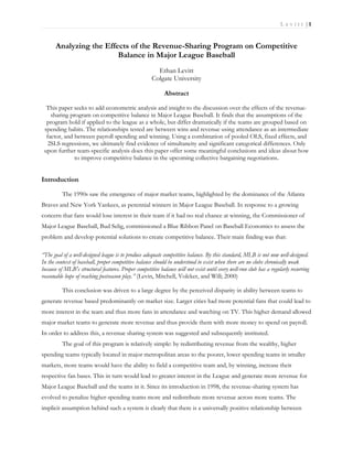
the 2010 season, provide evidence to the contrary. The correlation between winning and spending, as
measured in Figure 2, has been generally decreasing since the 1998 season, from .71 in 1998 to below .20 in
2010.
A verage MLB P ayroll (in millions of dollars) by Y ear
10 0
90
80
70
60
50
40
30
20
10
0
20 03 20 04 20 05 20 06 20 07 20 08 20 09 20 10
Figure 2 Figure 3
This diminution in a team’s ability to “buy” wins has coincidentally been met with a leveling out of
average payroll in the past three years, as seen in Figure 3. Many attribute this shift to the recent economic
downturns forcing teams to be more conservative in their spending habits. It has also been suggested that
improvements in scouting and developing younger players have allowed teams to make smaller investments
with greater upsides and hold on to these players for many years before they can begin to demand expensive
contracts or become free agents. While the philosophy of building a team around a young core of home-

8. Le vitt |8
grown talent and then filling in the remaining pieces with established veterans has been growing in popularity
and been met with great success over the past several seasons (see 2010 Rangers and Giants, 2008 Rays, and
even to a certain degree the 2009 Phillies), it is by no means the only philosophy employed. Other major
market teams like the Yankees, Red Sox, and Cubs have continued to sign players to enormous contracts and
have also been successful in their efforts. I believe this suggests two factors are at play.
The first relies on the work of Harry Raymond, who studied the draft pick-free agent compensation
system. He found that the current system of rewarding teams that lose free agents with premium draft picks
was outdated. Raymond used sabermetric statistics to quantify in a more definitive way the relationship
between the value of free agents and corresponding draft picks in terms of wins. His findings suggested that
the current system significantly overcompensates teams that lose a player to free agency, which encourages
teams to spend less money on free agents and focus more on developing young players.
The second factor draws on the findings of Solow and Krautmann (2005). Their article finds
statistically and economically significant evidence that what they call the “Marginal Revenue of a win”
increases as market size increases. I attribute this to a key distinction regarding the concept of payroll
efficiency. I believe that the concept of payroll efficiency has two interdependent components to it: 1)
spending the right amount on each player on the team, and 2) spending the right amount on total payroll. In
choosing the appropriate level of spending, a team must consider the expected return on a player. Professor
and author Vince Gennaro offers a dual approach to player valuation, asserting that a player has both
performance and marquee/franchise value. This is meant to adjust for the fact that signing a player like
Stephen Strasburg or Manny Ramirez has bigger implications than just what they do on the field since they
are incredibly marketable players. This is particularly true in major markets where advertising can have a
much greater impact. Thus, it can be argued that it is justified for major teams to spend more, or specifically
spend beyond performance value on a player since they will generate revenue for the franchise beyond the
revenue through wins. Since a key clause of the report used to create revenue sharing was “well-run club”, I
think it is important to distinguish that well-run can mean different things in different markets, in particular
that major market teams have reason to spend money not only on talent, but on fan appeal. This dichotomy
in spending strategy combined with improvements in scouting and player development may offer some
insight as to why major market teams have not dominated baseball in the past decade.
Attendance-Wins as an Indicator of Fan Interest
Of the many fundamental changes Major League Baseball has undergone over the past decades, one
of the most observable is in how it is viewed. The advent, expansion and success of MLB Advanced Media
(“MLBAM”), regional sports networks, and new theme park-like stadiums, has dramatically altered the
baseball fan’s landscape. However, one this has not changed over time: fans prefer winning teams to losing

9. Le vitt |9
teams. While there is substantial evidence to corroborate this claim, the recent indifference shown by the fans
of the Tampa Bay Rays during their AL East Division title illustrates that success does not guarantee
attendance in every market. Seeing as how the revenue sharing program was designed to benefit those specific
teams which suffer the most from a disinterested fan base, the system would only be working if the
“preference for winning” premise held true universally.
Surprisingly, while the league average for the slope of the attendance per wins relationship was always
positive and significant over time, it was not positive or significant for every team. This suggested external
factors were influencing attendance. While it is intuitive to create the two categories of fans (namely those
who are responsive to a winning team and those that aren’t), it is difficult to assess which fans (or cities)
belong in those categories. On the one hand are the teams that have had substantial variation in performance
and attendance over the past 8 seasons (this was the case for 12 of the teams in MLB). In these cases the
relationships were always positive and confirmed the long-standing assumption that winning brings in more
fans. However, three groups of outliers presented an interesting issue for the model. First, and I suppose
foremost, are the uncompetitive teams that didn’t draw many fans. For a number of these teams, there was
no significant fluctuation in wins, so it was impossible to tell if an improvement in their performance would
have generated the attendance spike that would be expected. Second was the category of teams with fans
who were so loyal they continued to attend in high numbers regardless of performance. Third is the category
of teams that performed well throughout all 8 years of the study and drew a high number of fans because of
it, so that any potential effects of a diminution in performance did not have a chance to occur. I believe that
any attempt to disallow those teams would be subjective and inappropriate (one cannot assume that because
it didn’t happen, it couldn’t), so I elected to keep them in the data set despite any clear method to control for
the varying conditions. It is a goal of my continued to research to develop a model that can accommodate
differences between markets more adequately with regards to attendance.
However, even solving this conundrum would not completely clarify the issue of how attendance
relates to winning. From an economic point view, a baseball team has a monopoly over tickets in that they are
the sole supplier of the product and control the prices. However, if a team cannot identify what the demand
for their tickets is, then they cannot set the “right” prices, whatever their conception of “right” (most likely
profit-maximizing) is. This is only further exacerbated by the fact that baseball teams charge multiple prices
for various ticket quantities and qualities (based on location in the stadium, giveaways, opponent, etc.). If
ticket prices are set too high, then they will prohibit fans from positively responding to a winning team by
attending more games.
It is important to note that not all winning teams are competitive teams, and not all competitive
teams necessarily win that many games. A team with a .500 winning percentage may be in the playoff hunt in
September one year while a team that ends up winning 90 games never really has a chance that same season.
Given that playoff contention is not based solely on the number of wins a team has but rather the number of

10. L e v i t t | 10
wins a team has relative to other teams in its division or in Wild Card race, I think future analysis would
benefit from studying whether fans are interested in seeing a winning team or a competitive team. One good
example of this the 82 win 2005 NL West Champion San Diego Padres that drew a proportionately high
number of fans relative to their win total.
One interesting observation associated with this relationship is that attendance has dropped the last
three years (Figure 4).
Average M LB Attendance
3 4 0 00
3 3 0 00
3 2 0 00
3 1 0 00
3 0 0 00
2 9 0 00
2 8 0 00
2 7 0 00
2 6 0 00
2 5 0 00
2003 2004 2005 2006 2007 2008 2009 2010
Figure 4
This is likely due to a combination of multiple factors including the general economic recession,
smaller stadiums, and higher ticket prices. Regardless of the explanation though, it is an important trend to
account for in looking at recent data since teams that maintained attendance levels actually increased relative
to the league. In addition, new stadiums always bring more fans to the ballpark and more interest to the team,
and that effect usually lasts a few years, though the effect can vary. Stadiums have been developed and built
with a greater frequency in the past decade than ever before. However, the new stadiums were not considered
when looking at changes in attendance and a method for accounting for differences in both size and age of a
ballpark should be addressed in future research.
Revenue-Attendance as an Indicator of Front Office Operations
This relationship was originally meant to connect the final dots between spending and earning, with
the assumption that the relationship between attendance and revenue would be similarly positive across all
teams. In the broader sense, the coefficient for this relationship is supposed to represent roughly how much a
team makes in additional total revenue from one fan per game. Using the financial reports (see Figure 5
below) as a sample to determine how much revenue from attendance comprises total revenue, I was able to
see a clear and distinct difference in revenue generation between teams depending on market size.

11. L e v i t t | 11
Figure 5
Pittsburgh Pirates LA Angels of Anaheim
2007 2008 2008 2009
Home Game
Receipts 103.21 100.12
(tickets) 34.42 32.13 43% 42%
% of total 25% 22%
42.97 45.998
Broadcasting 40.326 39.01
% of total 29% 27% 18% 19%
Total Revenue 138.636 145.99 237.87 240.824
Thus there is evidence that different markets rely on different factors to varying degrees, and a
program which seeks to neutralize those differences runs the risk of poorly accounting for how those
differences play out over time. Some teams are more dependent on attendance and local based revenue and
some on rely on general broadcast revenue. The goal of revenue sharing was to redistribute local revenues
from rich teams to poor teams in order to mitigate the difference. An interesting trend has developed over
the past three years which may have a substantial impact on how effective that method of revenue sharing is.
While revenues have continued to increase across MLB, attendance has dropped the past three years. This has
caused the coefficients for the Revenue-Attendance relationship to increase (Figure 6). This means that each
fan is technically generating more revenue in each subsequent year than in previous years. With this current
trend, the incentive seems to be heading towards maximizing profit per fan rather than maximizing the
number of fans, a dangerous path for Major League Baseball to be on.
Figure 6
R evenue (in millions ) pe r F an in A ttendanc e per G ame
0 .0 0 6
0 .0 0 5
0 .0 0 4
0 .0 0 3
0 .0 0 2
0 .0 0 1
0
2003 2004 2005 2006 2007 2008 2009
A corresponding decrease in the R-squared values of the year-by-year regressions indicates that this
may not explain the full story. Given that 8 of the 30 MLB teams have a negative coefficient for their
attendance-revenue relationship in our model, which suggests that for some teams higher average attendance
has a negative effect on revenue, our model does affirm that in general more fans leads to more revenue. The

12. L e v i t t | 12
examples of teams with decreasing attendance and increasing revenue suffer from a variety of factors which
alter their situation and make them outliers. With the interaction of all these various factors at play in
different ways and to different degrees, we turn to the conclusions that can be drawn.
Conclusion
Ultimately, having taken all these things into consideration, the fact remains that 25 teams in Major
League Baseball saw annual increases in revenue from 2003 to 2008 (including in 2008). Of these 25 teams,
none of them, not one, increased team payroll every year or increased in wins every year. While this was never
the assumption, it does provide sufficient evidence that there is more that goes into generating revenue than
spending and winning.
Given that as a foundation, this paper proposes three further conclusions pertaining specifically to
the revenue sharing program. First, it is rational for major market teams to adopt different spending strategies
than small market teams which includes signing elite players to lucrative deals. These are riskier investments
for teams and thus a “well-run” team will still have to make them efficiently. Second, the simultaneous
stadium-building boom (which draws more fans to the game) and media outlet expansion (which makes it
easier for people to watch games without coming to the ballpark) have stagnated the effects of the true
relationships between winning, attendance, and revenue. New stadiums will not continue to be built at their
recent rate and the effects of that as a revenue driver will diminish. As access to baseball media becomes
more widespread and accessible, teams will have to develop new ways to generate local revenue, which is
something revenue sharing cannot directly fix.
However, with the current Collective Bargaining Agreement set to expire in December 2011, there
are two prescriptions I would recommend be considered in the negotiations of the new agreement:
1) Restructure the draft pick- free agent compensation system. Small market teams
have been successful with growing regularity in the past few seasons by drafting
good players and developing them, but competitive teams need experience
players. If small market teams are reduced to signing old veterans to short
contracts because they cannot compete with the big spending teams financially,
then can not create the kind of long term performance consistency that is
necessary to win over fans.
2) Stay away from excessive reform and continue with the type of oversight that we
saw with the Florida Marlins. As many of the facts mentioned in this paper have
made clear, more teams are competitive than there were in the years leading up to
revenue-sharing. In the instances where that is not the case, the problem seems to
lie not with the program, but with the team.

13. L e v i t t | 13
Appendix
Equation 1 test -
. h a u sm n
a f i x e d r an d o m
C e f
o f i ci e nt s
( b) ( B) ( b- B ) s qr t ( di a g ( V_ b - V _B) )
f i x ed r a ndom Di f f e r en c e S. E .
wi n s 2 . 0 7 14 4 6 2 . 8 01 2 9 1 - . 7 2 9 84 4 4 .
wi n s 2 - 3 . 6 6 28 2 2 - 4 . 8 95 6 8 6 1 . 2 3 28 6 4 .
wi n s 3 2 . 0 8 26 9 2 2 . 7 79 7 1 9 - . 6 9 7 02 7 5 .
y e a r 1 1 . 8 99 5 8 1 1 . 93 5 2 5 - . 0 3 56 7 7 .
b = c o n si s t e nt u n d er Ho an d Ha; obt ai ne d f r om xt r e g
B = i nc ons i s t e nt unde r Ha , ef f i c i en t unde r Ho; obt ai ne d f r om xt r e g
T es t : H :
o di f f e r en c e i n c oe f f i c i e nt s not s y s t em t
a i c
c hi 2 (4 ) = ( b- B) ' [ ( V_ b - V_ B) ^ (- 1 ) ] ( b - B)
= - 7 . 84 c h i 2 < 0 = = > m de l
o f i t t e d o n t he s e
da t a fa i l s t o m et
e t h e a s y m t o
p t i c
a s s u m t
p i o ns of t he Ha u sm a n t e s t ;
s e e s ue s t f o r a ge n e r a l i z e d t e s t
Equation 4 tests -
Ramsey RESET test using powers of the fitted values of revenue
Ho: model has no omitted variables
F(3, 201) = 8.53
Prob > F = 0.0000
Variable | VIF 1/VIF
-------------+----------------------
wins2 | 19432.69 0.000051
wins3 | 5471.62 0.000183
wins | 4411.68 0.000227
attend | 1.29 0.772630
year | 1.04 0.964681
-------------+----------------------
Mean VIF | 5863.66
150
100
Residuals
50
0
-50
100 150 200 250 300
Fitted values
DM test
. r e g r e v e nue wi ns wi n s2 wi n s3 y e a r a t t en d y h at l
So u r c e SS df MS Nu m b e r of obs = 2 1 0
F( 6 , 2 0 3 ) = 63 . 0 7
M ode l 3 03 4 9 8 . 8 9 4 6 5 0 5 8 3. 1 4 9 Pr o b > F = 0 . 0 0 0 0
Res i d u a l 1 62 8 1 8 . 3 8 7 2 0 3 8 0 2 . 06 1 0 2 R- s q u a r ed = 0 . 6 5 0 8
Ad j R- s q ua r e d = 0 . 6 4 0 5
Tot a l 4 66 3 1 7 . 2 8 1 2 0 9 22 3 1 . 18 3 1 6 Ro ot M SE = 2 8. 3 2 1
re v e nue Co ef . St d. Er r . t P> | t | [ 9 5 % Co n f . I nt e rv a l ]
wi n s 22 . 0 7 92 6 1 1 . 7 0 12 1 . 8 9 0 . 0 61 - . 9 9 2 21 3 3 4 5 . 15 0 7 4
wi n s 2 - 34 . 7 4 81 2 15 . 3 0 0 04 - 2 . 2 7 0 . 0 24 - 6 4 . 91 5 5 - 4 . 5 80 7 4 2
wi n s 3 17 . 4 9 78 3 6. 6 2 1 1 13 2 . 6 4 0 . 0 09 4 . 4 4 28 5 1 3 0 . 5 5 2 8
y e a r 8. 6 3 2 69 1 6. 4 2 0 2 11 1 . 3 4 0 . 1 80 - 4 . 0 26 1 6 2 1 . 29 1 5 4
a t t e n d 10 0 . 2 48 3 82 . 3 8 2 75 1 . 2 2 0 . 2 25 - 6 2 . 1 87 3 5 2 6 2 . 6 8 3 9
y ha t l . 2 2 3 6 03 9 . 6 1 3 4 0 36 0 . 3 6 0 . 7 16 - . 9 8 5 85 5 5 1 . 4 33 0 6 3
_ c o n s - 17 7 0 2 . 4 9 12 9 0 4 . 92 - 1 . 3 7 0 . 1 72 - 4 3 1 4 7. 3 6 7 7 4 2. 3 8 5

14. L e v i t t | 14
Equation 5 tests-
Ramsey RESET test using powers of the fitted values of wins
Ho: model has no omitted variables
F(3, 201) = 0.94
Prob > F = 0.4242
20
0
Residuals
-20
-40
70 80 90 100
Fitted values
Equation 6 tests -
Hausman test on 2SLS
C e f
o f i ci e nt s
( b) ( B) ( b- B ) s qr t ( di a g ( V_ b - V _B) )
s l s ol s Di f f e r en c e S. E .
wi n s 8 9 . 4 56 8 4 2 2 . 71 8 3 3 6 6 . 7 38 5 1 1 4 0 . 19 5 3
wi n s 2 - 1 2 5 . 79 5 3 - 3 5 . 25 4 1 7 - 9 0 . 5 41 1 5 1 7 8 . 7 7 3
wi n s 3 6 1 . 01 3 6 1 7 . 65 3 1 3 4 3 . 3 60 4 7 7 5 . 1 12 3 8
y e a r 1 3 . 6 9 6 1 0 . 94 4 7 8 2 . 7 5 12 1 6 2 . 7 9 75 2 6
a t t e n d - 5 7 . 1 38 1 6 1 2 9. 9 4 2 - 1 8 7 . 08 0 1 8 0 . 2 05 1 8
b = c on s i s t en t un de r Ho a nd H ;
a obt a i ne d f r om i v r e gr e s s
B = i nc ons i s te nt un de r Ha, e f f i c i e nt unde r Ho ; obt a i ne d f rom r e g r e s s
T es t : H :
o di f f e r en c e i n c oe f fi c i e nt s not s y s t em t
a i c
c hi 2 (5 ) = ( b- B) ' [ ( V _ b - V _ B) ^ (- 1 ) ] ( b- B)
= 17 . 3 7
Pr o b > c hi 2 = 0 . 0 0 3 8
Single Regression Results -
Revenue in
Avg. number Millions per
of fans in avg number of
Wins per Million thousands per fans in
Team Spent on Payroll Win thousands Product of Three = Rate of Return
Philadelphia Phillies 0.177 1163.8 0.0055 1.1329593
Tampa Bay Rays 0.6258 245.1 0.0055 0.84360969
St. Louis Cardinals 0.758 158.06 0.0067 0.802723516
Milwaukee Brewers 0.2503 657.17 0.0042 0.690856534
Los Angeles Angels of
Anaheim 0.497 129.9 0.0086 0.55521858
Baltimore Orioles -0.1709 931.93 -0.0029 0.461873827 double neg
New York Yankees -0.131 -651.44 0.0042 0.358422288 double neg
Oakland A's -0.2245 361.6 -0.0044 0.35718848 double neg

15. L e v i t t | 15
Detroit Tigers 0.234 348.09 0.0029 0.236213874
Texas Rangers -0.62 173.45 -0.002 0.215078 double neg
Colorado Rockies 0.223 223.53 0.0038 0.189419322
Minnesota Twins 0.071 232.7 0.0093 0.15365181
Seattle Mariners -0.416 178.81 -0.0016 0.119015936 double neg
Toronto Blue Jays 0.1236 140.09 0.0068 0.117742843
Boston Red Sox -0.051 -99.6 0.0215 0.1092114 double neg
San Francisco Giants -0.0072 33.169 -0.0065 0.001552309 double neg
Cincinnati Reds 0.147 -78.84 -0.005 0.0579474
Washington Nationals -0.2711 -49.708 0.0038 0.051208187
Arizona Diamondbacks -0.2977 44.216 -0.0024 0.031591448
Los Angeles Dodgers 0.196 14.063 0.0103 0.028390384
Pittsburgh Pirates 0.193 28.803 0.0014 0.007782571
Chicago White Sox -0.0596 -15.757 0.0045 0.004226027
Kansas City Royals 0.0116 74.83 0.0003 0.000260408
Atlanta Braves 0.0072 -89.014 0.0065 -0.004165855
Florida Marlins 0.12 51.979 -0.0013 -0.008108724
San Diego Padres -0.426 28.693 0.0017 -0.020779471
Chicago Cubs -0.03 50.931 0.0215 -0.032850495
Houston Astros -0.5242 147.8 0.0028 -0.216934928
New York Mets -0.121 580.85 0.0039 -0.274103115
Cleveland Indians -0.207 240 0.0056 -0.278208
Bibliography and References
Baseball Almanac, found at www.baseball-almanac.com.
Baseball Refereece, found at www.Baseball-reference.com.
Bradbury, J.C. The Baseball Economist: The Real Game Exposed. New York: Dutton, 2007.
Bradbury, J.C. “Revenue Sharing, Incentives, and Competitive Balance” www. Sabernomics.com.
September 1, 2010.
Brown, Maury. “Will leaked MLB financials alter Revenue-Sharing?” Fangraphs. August 25, 2010.
http://www.fangraphs.com/blogs/index.php/will-leaked-mlb-financials-kill-revenue-sharing/
Elanjian, Michael R. and Dessislava A. Pachamanova. “Is Revenue Sharing Working for Major
League Baseball? A Historical Perspective”. The Sport Journal. Volume 12, No. 2.

16. L e v i t t | 16
http://www.thesportjournal.org/article/revenue-sharing-working-major-league-baseball-historical-
perspective
Futterman, Matthew. “The Year Money Didn’t Matter”. Wall Street Journal. September 16, 2010.
http://online.wsj.com/article/SB10001424052748703743504575493942146685242.html
Gennaro, Vince. Diamond Dollars: The Economics of Winning in Baseball. Hingham, Ma.: Maple
Street Press, 2007.
Gustafson, Elizabeth and Lawrence Hadley. “Revenue, Population, and Competitive Balance in
Major League Baseball”. Contemporary Economic Policy. Volume 25, No. 2. April 2007.
Hakes, Jahn K., and Raymond D. Sauer 2006. "An Economic Evaluation of the Moneyball
Hypothesis." Journal of Economic Perspectives, 20(3): 173–186.
Jacobson, David. “The Revenue Model: Why Baseball is Booming”. Bnet website. July 11, 2008.
http://www.bnet.com/article/the-revenue-model-why-baseball-is-booming/210671
Levin, R. C., Mitchell, G. J., Volcker, P. A., & Will, G. F. (2000). The Report of the independent
members of the commissioner's Blue Ribbon Panel on baseball economics. Retrieved December 10, 2010
from Major League Baseball Website: http://www.mlb.com/mlb/downloads/blue_ribbon.pdf
Solow, J., and A. C. Krautmann. “Leveling the Playing Field or Just Lowering Salaries?” Working
Paper, University of Iowa, 2005.
Zimbalist, Andrew. May the Best Team Win: Baseball Economics and Public Policy. Washington D.C. : The
Brookings Institution, 2003.