lines and angles in radiology

1. Roentgenometrics
S.THIYAGARAJAN
 Application of standard lines and measurements to radiographs
 Allows the detection of subtle abnormalities
 Assists in avoiding misdiagnosis
 Comparison of studies is facilitated
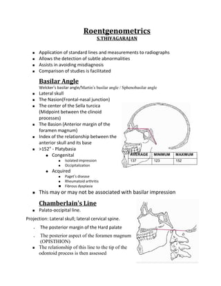
Basilar Angle
Welcker’s basilar angle/Martin’s basilar angle / Sphenobasilar angle
 Lateral skull
 The Nasion(Frontal-nasal junction)
 The center of the Sella turcica
(Midpoint between the clinoid
processes)
 The Basion (Anterior margin of the
foramen magnum)
 Index of the relationship between the
anterior skull and its base
 >152° - Platybasia
 Congenital AVERAGE MINIMUM MAXIMUM
 Isolated impression 137 123 152
 Occipitalization
 Acquired
 Paget’s disease
 Rheumatoid arthritis
 Fibrous dysplasia
 This may or may not be associated with basilar impression
Chamberlain’s Line
 Palato-occipital line.
Projection: Lateral skull; lateral cervical spine.
 The posterior margin of the Hard palate
 The posterior aspect of the foramen magnum
(OPISTHION)
 The relationship of this line to the tip of the
odontoid process is then assessed

2.  Tip of the odontoid process should not project above this line
 Normal variation of 3 mm above this line may occur
 A measurement of ≥7 mm is definitely abnormal.
 An abnormal superior position of the odontoid
 Basilar impression
 Platybasia
 Atlas occipitalization
 Bone-softening diseases of the skull base
 Paget’s disease
 Osteomalacia
 Fibrous dysplasia
 Rheumatoid arthritis
McGregor’s Line (Basal line)
Projection: Lateral skull; lateral cervical spine.
 Postero superior margin of the hard palate
 Most inferior surface of the occipital bone
 The relationship of the odontoid apex to this line
is examined
 > 8 mm in males
 > 10 mm in females
 In children younger than 18 years, these maximum values diminish with
decreasing chronologic age.
 McGregor’s line appears to be the most accurate and reproducible
 Abnormal superior position of the odontoid
 Basilar impression
Macrae’s Line
 Foramen magnum line
 The Basion (anterior margin of the
foramen magnum)
 Posterior (Opisthion) margins of the
foramen magnum
 The inferior margin of the occipital bone
should lie at or below this line

3.  In addition a perpendicular line drawn
through the odontoid apex should intersect
this line in its anterior quarter
 If the inferior margin of the occipital bone is
convex in a superior direction and/or lies
above this line, then basilar impression is
present.
 If the odontoid apex does not lie in the
ventral quarter of this line
 Dislocation of the atlanto-occipital joint
 Fracture
 Dysplasia of the dens
Digastric Line (Biventer line)
Projection: AP open mouth
 The digastric groove medial to the base of the mastoid process
 The vertical distance to the odontoid apex and atlanto occipital joints is
measured
Measure Average (mm) Minimum (mm) Maximum (mm)
Digastric line-odontoid apex 11 1 21
Digastric line-atlanto-occipital 12 4 20
joint
 Both measurements will decrease in
basilar impression
• Platybasia
• Atlas occipitalization
• Bone-softening diseases of the
skull base
• Paget’s disease
• Osteomalacia
• Fibrous dysplasia
• Rheumatoid arthritis
Occipitoatlantal alignment
 Projection: Lateral skull.
 Two lines are constructed

4. 1. Foramen magnum line (FML) is drawn along the inferior margin of the
occiput (MACRAE’S LINE)
2. Atlas plane line (APL) is drawn
through the center of the anterior
tubercle and the narrowest portion of
the posterior arch of atlas
 The FML and APL should be parallel.
 Divergence of the FML and APL
anteriorly suggests anterior-superior
malposition of the occiput
 Divergence of the lines posteriorly
suggests posterior-superior malposition
of the occiput
Other method
 The anterior margin of the foramen magnum should line up with the dens.
 A line projected downward from the dorsum sellae along the clivus to the
basion should point to the dens.
Wachenheim's line
 The posterior margin of foramen magnum
should line up with the C1 spinolaminar
line.
 Power ratio :The ratio of Basion -
spinolaminar line of C1 to Opisthion -
posterior cortex of C1 anterior arch
normally ranges from 0.6 to 1.0, with the
mean being 0.8. A ratio greater than 1.0
implies anterior cranio-cervical dislocation.
Sella Turcica Size
The greatest AP diameter and the greatest vertical diameter
Diameter Average (mm) Minimum (mm) Maximum (mm)
Anteroposterior 11 5 16
Vertical 8 4 12

5.  Small sella
Normal variant
Hypopituitarism (long after Sheehan's)
Microcephaly
Myotonic dystrophy
Prader-Willi-Lambert syndrome
Cockayne syndrome
Dystrophia myotonica
 Enlarged sella
Pituitary neoplasm
Empty sella syndrome
Extrapituitary mass
 Neoplasm
 Aneurysm
Normal variant
 J shaped sella
Elongated sella with shallow anterior
convexity which represents exaggerated of sulcus chiasmaticus
 Normal variant
 MPS
 Achondroplasia
 Chronic hydrocephalus
 Optic chiasmatic glioma
 Osteogenisis imperfecta
 Neurofibromatosis
Atlantoaxial "overhang" sign
AP open-mouth projection
 Lateral margin of the lateral masses of
atlas should not appear more lateral than
the superior articular processes of axis
 If the lateral margin of the atlas lateral mass lies

6. lateral to the lateral axis margin,
 Radiologic sign of
 Jefferson’s fracture
 Odontoid fracture
 Alar ligament instability
 Rotatory atlantoaxial
subluxation
 Mild degree of overhanging may be a
normal variant
Atlantodental Interspace
 Atlas-odontoid space, predental
interspace, atlas-dens interval
 Projection: Lateral neutral; flexion-
extension cervical
Age Minimum Maximum
spine. (mm) (mm)
 The distance measured is Adults 1 3
between the posterior margin of
Children 1 5
the
 anterior tubercle and the anterior
surface of the odontoid
Decreased space
Advancing age (Degenerative joint disease of the
atlantodental joint)
Widened space with reduction in the neural
canal size
Trauma
Occipitalization
Down’s syndrome
Pharyngeal infections (Grisel’s disease)
Inflammatory arthropathies
Ankylosing spondylitis
Rheumatoid arthritis
Psoriatic arthritis
Reiter’s syndrome
Cervical Gravity Line
 A vertical line is drawn through the apex of
the odontoid process

7.  This line should pass through the C7 body
 Gross assessment of where the
gravitational stresses are acting at the
cervicothoracic junction.
Stress Lines of the Cervical
Spine
 Ruth Jackson’s lines
 Projection: Lateral cervical spine (flexion,
extension)
 Two lines are constructed on each film
1) The first line is drawn along the
posterior surface of the axis
2) The second line is drawn along
the posterior surface of the C7
body until it intersects the axis
line
 Normal Measurements
 Flexion - lines should intersect at the level
of the C5-C6 disc or facet joints.
 Extension - lines should intersect at the
level of the C4-C5 disc or facet joints.
 The intersection point represents the
focus of stress when the cervical spine is
placed in the respective positions
 The point of intersection does not appear
to correlate with the level of degenerative
disc disease
 Muscle spasm, joint fixation, and disc
degeneration may alter the stress point.
Cervical Lordosis
Visual assessment (Subjective)
 On the lateral cervical projection
 Well maintained anterior convexity
is lordosis
 Exaggerated anterior convexity is hyperlordosis

8.  Slight anterior convexity hypolordosis
 Lack of curvature is alordosis
Posterior convexity is kyphosis
 Altered cervical lordosis
 Trauma
 Degeneration
 Muscle spasm
 Aberrant inter-segmental mechanics
Depth method
Lateral cervical projection
 A line is drawn from the tip of the odontoid
process to the posterior surface of C7
 A horizontal measure is taken from the
vertical line to the posterior surface of the
C4 body (X)
 The average depth is 12 mm
 Negative – Kyphosis
 Largest values – Hyperlordosis
 The depth method provides a more accurate assessment of cervical lordosis
Angle of curve
Lateral cervical projection
 A line is drawn connecting the anterior
and posterior tubercles of the atlas
 Second line is drawn along the inferior
endplate of C7
 Perpendicular lines are drawn from the
atlas and C7 lines, and their angle of
intersection is recorded as the cervical
lordosis (X°)
 The average value is 40 degrees
 Negative – kyphosis
 Large – hyperlordosis
 Less accurate than the depth
method. Because the measurements
depend only on CI and C7
Prevertebral Soft Tissues

9.  The soft tissue in front of the vertebral bodies and
behind the air shadow of the pharynx, larynx, and
trachea is measured
 The bony landmarks
 Anterior arch of the atlas
 Inferior corners of the axis & C3
 Superior corner of C4
 Inferior corners of C5, C6, and C7
 C2-C3 - RPI
 Behind the larynx (C4-C5) - RLI
 Behind the trachea (C5-C7) - RTI.
Widening
 Post-traumatic hematoma
 Retropharyngeal abscess
 Neoplasm from the adjacent bone and soft tissue structures.
Level Flexion (mm) Neutral (mm) Extension (mm)
C1 11 10 8
C2 6 5 6
C3 7 7 6
C4 7 7 8
C5 22 20 20
C6 20 20 19
C7 20 20 21
Spinolaminar junction line
Posterior Cervical Line, arch-body line.
 Projection: Lateral cervical spine
(neutral, flexion, extension).
 The cortical white line of the
spinolaminar junction identified at
each level C1 to C7
• Each spinolaminar junction will be
curved slightly anteriorly from
superior to inferior

10. • For consistency, the most anterior part of the convexity is
compared between levels
 Discontinuous at any level
 Anterior or posterior displacement
 This line is especially useful for
detecting subtle odontoid fractures
and atlantoaxial subluxation
(anterior)
 A disruption in the middle to lower
cervical spine may also be a sign of
anterolisthesis, retrolisthesis, or
frank dislocation.
Cervical Spinal Canal
Projection: Lateral cervical (neutral,
flexion, extension)
 The sagittal diameter is measured
from the posterior surface of the
midvertebral body to the nearest
surface of the same segmental
spinolaminar junction line
Level Average (mm) Minimum (mm) Maximum (mm)
C1 22 16 31
C2 20 14 27
C3 18 13 23
C4 17 12 22
C5 17 12 22
C6 17 12 22
C7 17 12 22
Narrowing of the canal (stenosis) < 12 mm
Significance

11.  If degenerative posterior osteophytes are
present, the measurement can be made
from their tip to examine the magnitude of
the stenotic effect. The degree of stenosis
from these spurs is best measured on
extension films
 An abnormally widened canal may be
associated with a spinal cord neoplasm or
syringomyelia.
 The most accurate measurement is by the ratio
of the sagittal dimension of the canal and
vertebral body (canal to body ratio, Pavlov’s
ratio)
 A ratio of less than 0.82 is significant for spinal
stenosis. The benefit of this method is that it
removes the effects of radiographic
magnification.
Cervical, thoracic, and
lumbar endplate lines
 On the lateral cervical projection, lines arc
drawn along the inferior endplate of the
C2-T1 vertebrae and extended posteriorly
to the cervical spine
 The cervical endplate lines should all
intersect at a common point located
posterior to the spine
 Lack of convergence
 Normal lordotic cervical spine
curve
 Intersegmental malpositions
 Lines that cross closely to the spine
 Extension malposition of the
superior segment
 Lines that diverge sharply
 flexion malposition of the
superior segment.

12.  Frontal cervical, thoracic, and lumbar projections
 Lines are drawn to approximate the inferior vertebral endplates
 The lines at adjacent levels should be parallel
 Divergence of the endplate lines
 Lateral flexion malposition opposite the side of divergence
Cervical, thoracic, and lumbar vertebral
rotation
Body width method
 Distance from the lateral margins
of the vertebral bodies to the
origin of the spinous process
should be equal bilaterally.
 Distances not equal
 Vertebral rotation
Spinous process deviation to the side of the smaller distance.
Pedicle method
Frontal projection
 The appearance of the pedicle
shadows may suggest vertebral
rotation
 It is expected the pedicle shadows
demonstrate bilateral symmetry
 If the width of a pedicle shadow
appears narrower than the
contralateral pedicle shadow, it
suggests
 Segmental rotation with the
spinous process deviated to the
side of the narrower pedicle
shadow
 Posterior vertebral body

13. rotation to the side of the wider pedicle shadow
Cervical, thoracic, and lumbar vertebral sagittal
alignment
George's line
Lateral projections
 Curvilinear line is drawn along
the posterior surfaces of the
vertebral bodies
 The curve should maintain a
smooth contour throughout
the spinal region without segmental disruption.
 Disruption
 Segmental anterolisthesis
 Retrolisthesis
 Disruptions at multiple consecutive levels
 Normal flexion and extension patterns.
 However, the adjacent posterior body lines should not demonstrate more than 3 mm of
net translation in a comparison of the flexion and extension radiographs
Barge's "e" space
Lateral lumbar projection
 Lines are drawn along the superior and inferior vertebral endplates of each
segment
 Lines perpendicular to each endplate line are then drawn and extended
across the intervertebral disc space.
 The distance between the perpendicular lines at the inferior end- plate of
each lumbar segment is
measured as the "e" space
 The space should not exceed
3 mm
 Larger Barge's "e" space
 Retrolisthesis of the
segment above
 Negative values indicate

14.  Anterolisthesis
Visual method
 Segmental retrolisthesis
 Intervertebral disc degeneration (osteophytes, eburnation, reduced
disc space, Schmorl's nodes, endplate irregularity)
 The lowest segment of a "stack" of three or more vertebrae that do
not contribute to a sagittal curvature may be posterior
 The lowest involved segment of
three or more consecutive
segments that appear to be flexed
or extended during neutral patient
posture may be posterior
 Segmental rotation in a coronal
plane that produces an hourglass
appearance
 Narrowed sagittal diameter of the
intervertebral foramen
 Visual disparity of segmental
alignment when comparing the
margins of adjacent vertebrae
 Retrolisthesis of L5 is often seen as a
normal variant, accompanying short pedicles
Cervical toggle analysis
Atlas tilt
Lateral cervical projection
 Three lines are constructed
 Occipital condyle line (OCL) is
drawn along the base of the
occipital condyles
 Atlas plane line (APL) is drawn
through the center of the anterior
tubercle and the narrowest portion
of the posterior arch of the atlas
 Listing line (LL) is drawn parallel to
the occipital condyle line and

15. through the narrowest portion of the posterior arch of the atlas.
 The atlas plane line should be 4 degrees above the listing line
 APL > 4 degrees above the listing line
 Superior malposition of the atlas
 APL < 4 degrees
 Inferior malposition of atlas
Atlas laterality
 4 lines are constructed:
 Horizontal ocular orbit line (OOL) is drawn through similar matched points
of the orbits
 Superior basic line (SBL) is drawn
parallel to the OOL through the tip of
the most superior occipital condyle
 Inferior basic line (IBL) is drawn
through the inferior tips of the
lateral masses
 Vertical median line (ViML) is drawn
perpendicular to the OOL and
through the center of the foramen
magnum
 The distances between the inferior
lateral tip of each lateral mass and
the VML should be equal.
 The atlas is lateral toward the side of
the greater measurement when the
distances between the lateral
inferior tip of each lateral mass and
the VML are not equal
 In addition, the SBL and IBL lines are
thought to converge to the side of
atlas laterality 70% of the time
Atlas rotation
 On a cervical film whose projection is directed vertical to the atlas (base
posterior)
 Two lines are constructed

16.  Transverse atlas line (TAL) is drawn through the transverse foramen
bilaterally
 Perpendicular skull line (PSL) is drawn through points representing the
centers of the nasal septum and the basal process of the occiput
 The angle of intersection of the two lines should be approximately 90
degrees.
 The atlas is rotated posteriorly on the side of the larger angle
created by the intersection of the PSL and TAL.
 In addition, 70% of the time the atlas is posteriorly rotated to the
side of the diverging superior basic line (SBL) and inferior basic
line (IBL) on the frontal open mouth projection.
ATLAS MALPOSITION
Frontal open-mouth projection
 Four lines are constructed
 Ocular orbit line (OOL) is drawn
through a set of similar points of the
orbit
 Superior basic line (SBL) is drawn
bilaterally through the jugular
processes
 Inferior basic line (IBL) is drawn
through the lateral inferior tip of both lateral masses
 Vertical median line (VML) is drawn perpendicular to the OOL through the
center of the foramen magnum
 VML should approximate the center of the odontoid process base
 If the VML does not bisect the odontoid, the axis is laterally malpositioned
to the side opposite the VML.
 In addition, the center of the odontoid process base is compared with the
center of the spinous process to assess for possible spinous deviation.
 The direction and magnitude of spinous process lateral malposition may be
different from the lateral malposition of the axis body (i.e., the body of the
axis may be exhibit right laterality with left spinous deviation).

17. Cobb’s Method of Scoliosis Evaluation
Cobb-Lippman method
 Projection: AP spine.
End vertebrae
 Last segment that contributes to the spinal
curvature.
 Extreme ends of the scoliosis, where the
endplates tilt to the side of the curvature
concavity
Endplate lines
 On the superior end vertebra, a line is drawn
through and parallel to the superior endplate
 On the inferior end vertebra, a line is constructed
in a similar manner through and parallel to the
inferior endplate
 This is the preferred method in scoliosis
assessment
 In patients with double scoliotic curves each component should be
measured.
 5° progression of a scoliosis between two successive radiographs is
considered significant

 Curvatures < 20° - No bracing or surgical intervention
 Patient between 10 and 15 years of age, careful monitoring should be
implemented to assess for progression of 5° or more in any 3-month period.
 Curves between 20° and 40° - Bracing / Surgical intervention
 Curvature progression in an immature spine, or curvature in excess of 40° -
Surgical intervention
Risser-Ferguson Method of Scoliosis Evaluation
AP spine.
 Apical vertebra
 Most laterally placed segment in the curve
Vertebral body center
 For each end vertebra and apical segment diagonals are drawn from
opposing corners of the body to locate the body center
 Connecting line

18.  Two lines are constructed connecting the body
centers of the apical segment with each end
vertebra, and the resultant angle is measured
 This method gives values approximately 25%
lower than those of Cobb’s method (10°)
 Advocated its use for larger curves
Coupled spinal motion sign
 Spinal motion is not pure and occurs in directions other
than the primary direction of movement
 For example, on frontal cervical, thoracic, or lumbar
lateral bending projections, the lateral tilting of each
vertebra is accompanied by concurrent vertebral rotation
 In the cervical and upper thoracic region the spinous
processes rotate to the convexity of the curve
 In the lumbar and lower thoracic region the
spinous processes rotate to the concavity of the
curve
 The amount of coupled motion may be small and therefore radiographically
imperceptible.
 Alteration of the normal coupled motion occurs with aberrant
intersegmental mechanics, muscle spasm, and vertebral fusion
Interpedicular Distance
 Coronal dimension of the spinal canal
 Projection: AP cervical spine, thoracic
spine, and lumbar spine.
 The shortest distance between the
inner convex cortical surfaces of the
opposing segmental pedicles is
measured
Spinal Level Maximum (mm)
Cervical spine 30
Thoracic spine 20
L1 TO L3 25
L4, L5 30

19.  This is a useful measurement applied in
the evaluation of spinal stenosis,
congenital malformation, and intraspinal
neoplasms
 The maximum interpediculate distance
may be increased as a result of pedicular
erosion from an expanding spinal cord
tumor (Elseberg-Dyke sign)
Thoracic Cage Dimension
Straight back syndrome evaluation
 Projection: Lateral chest.
 The distance between the posterior
sternum and the anterior surface of
the T8 body is measured
Normal Sagittal Dimensions of the Thoracic Cage
Sex Average (cm) Minimum (cm) Maximum (cm)
Male 14 11 18
Female 12 9 15
Sagittal Dimensions of the Thoracic Cage in Straight Back Syndrome
Sex Average (cm) Minimum (cm) Maximum (cm)
Male 11 9 13
Female 10 8 11
Thoracic Kyphosis
Lateral thoracic spine
 A line is drawn parallel to and through the
superior endplate of the T1 body
 A similar line is drawn through the inferior
endplate of the T12 body.
 Perpendicular lines to these endplate lines are
then constructed
 Intersecting angle is measured

20.  Physiologic anterior vertebral body
wedging accounts for the natural
kyphotic curvature of the thoracic spine
 Normal anterior wedging for each
vertebral body is 4-5° or 2-3 mm
 The wedging increases by almost 1 mm
for each successive level, with
approximately 45° of thoracic kyphosis
accounted for by this wedging
 Increased kyphosis
 Old age
 Osteoporosis
 Scheuermann’s disease
 Congenital anomalies
 Muscular paralysis
 Cystic fibrosis
 Reduction in kyphosis
 straight back syndrome
Lumbar Intervertebral Disc Angles
 Lines are drawn through and parallel to each
lumbar body endplate
 The lines are extended posteriorly until they
intersect
 Intersecting angle is measured
Normal Values for Lumbar Intervertebral Disc Angles
Disc Level Average Angle (°)
L1 8
L2 10
L3 12
L4 14
L5 14
Mean angle alteration
Antalgia
Muscular imbalance

21. Improper posture
Facet syndrome - Increased Angle
Acute discal injuries - Decreased Angle
Lumbar Intervertebral Disc
Height
Lateral lumbar spine
 Visual assessment
 Disc height compared with the adjacent
levels
 Past experience
Hurxthal’s method
 The distance between the opposing endplates
at the midpoint between the anterior and the
posterior vertebral body margins is measured.
Farfan’s method
 Anterior disc height (A) & posterior disc height (P) are measured and expressed as a
ratio to disc diameter (D)
 These two ratios are then reduced to a ratio of each other
Lumbar spine - normal disc ratios increase
LI 0.17
L2 0.18
L3 0.20
L4 0.25
L5 0.28
 When segmental rotation is > 40° or lateral
flexion is > 20°, these methods become
unreliable.
 Decreased disc height
 Disc degeneration
 Post surgery
 Post chemonucleolysis
 Infection
 Congenital hypoplasia

22. Hadley’s S Curve
Lumbar facet curve
 Projection: Oblique, AP lumbar spine
 Curvilinear line is constructed along the inferior margin of the transverse
process and down along the inferior articular process to the apophyseal
joint space
 Line is then continued across the articulation to connect with the outer
edge of the opposing superior articular process
 The resultant configuration of this line will look like the letter S
 The key region of the S is the normally smooth transition across the joint
space
 Abrupt interruption in the smooth contour of this line may indicate facet
imbrication (subluxation)
Lumbar Gravity Line
 The center of the L3 body is located by
intersecting diagonals from opposing body
corners
 A vertical line is constructed through center
point
 Relationship to the upper sacrum is assessed
 Center of gravity of the trunk passes through
the center of the L3 body and continues
vertically to intersect the sacral base
 Normally the vertical line will pass through
the anterior third of the sacral base.
 If this line passes anterior to the sacrum by >
0.5 inch (> 10 mm), an increase in shearing
stresses in an anterior direction between the lumbosacral apophyseal joints
may be occurring.
 Conversely, it has been suggested that a posterior shift in this gravity line
may indicate increased weight bearing forces on these same lumbosacral
joints that may also be active in the production of low back pain

23. Van Akkerveeken’s
Measurement of
Lumbar Instability
 Projection: Lateral lumbar spine
(neutral, flexion, extension).
 Two lines are drawn through and
parallel to opposing segmental
endplates until they intersect
posteriorly.
 The distance from the posterior
body margins to the point of
intersection is then measured.
 Alternatively, the displacement can
be assessed by measuring the offset
in the opposing body corners
Normal Measurements
 There should be < 1.5 mm displacement, as
determined by either measurement method
 If there is > 1.5 mm (3mm) difference in
measurement, then it is likely that nuclear,
annular, and posterior ligament damage at the
displaced segment is present
Lumbar Lordosis
 Lumbar curve, lumbar spinal angle, lumbar angle
 Projection: Lateral lumbar spine.
 Line is drawn through and parallel to the superior
endplate of the first lumbar segment
 Second line is drawn through the superior endplate of the first sacral
segment
 Perpendiculars are then created, and the angle at their intersection is
measured
 A wide variation exists within normal individuals.
 The average appears to be 50-60°

24. Lumbar spinal canal
Eisenstein's method
Lateral lumbar projection
 Line is drawn connecting the tips of the
superior and inferior articular processes of the
same segment
 The canal width (x) is expressed as the distance
from the posterior body margin to the middle
portion of the facet line
 The canal dimension should not fall below 15
mm (although some use 14 mm or 12 mm as
the cutoff)
 Smaller measurements may indicate spinal stenosis
 Spinal stenosis is more accurately assessed on axial MRI and CT images
RATIO METHOD
Frontal lumbar projection
 Interpedicular distance is multiplied
by sagittal width
 Coronal width of the vertebrae is
multiplied by the sagittal width
 The product of the two canal
measures is divided by the product
of the two vertebral measures,
expressing the canal size as a ratio of
the vertebral body
 In the lumbar spine, the canal ratio should not fall below 1:3
Meyerding’s Grading Method in Spondylolisthesis
 The superior surface of the first
sacral segment is divided into four
equal divisions. The relative
position of the posterior inferior
corner of the L5 body to these
segments is then made

25.  The posterior inferior corner of the L5 body should be aligned with the
posterior-superior corner of the first sacral segment.
 The same assessment can be applied to other spinal levels by dividing the
superior endplate of the segment below the spondylolisthesis into four
equal spaces.
 In spondylolisthesis, > 12° dynamic angulation or 8% translation on flexion-
extension views is considered evidence of instability
 The degree of anterolisthesis of the affected vertebral body can be
categorized according to the division in which the posterior-inferior corner
of the body lies
Grade 1 The posterior-inferior corner is aligned within the first division
Grade 2 The posterior-inferior corner is aligned within the second division
Grade 3 The posterior-inferior corner is aligned within the third division
Grade 4 The posterior-inferior corner is aligned within the fourth division
 If the vertebral body has completely
slipped beyond the sacral promontory, the
condition is called spondyloptosis
Lumbosacral Angle
Two lines
 First, a horizontal line is made parallel to
the bottom edge of the film
 Second, an oblique line is drawn through
and parallel to the sacral base.
Normal Values for Lumbosacral Angle
Position Average Standard Minimum Maximum
(°) Deviation (°) (°)
Upright 41 ±7 26 57

26. Sacral angle / Barge's
angle
 The angle of the superior margin of
the sacrum from the horizontal plane,
measured in the sagittal plane
 lumbar lordosis increased if the sacral
angle increased
Ullmann’s Line
 Garland-Thomas line, right-angle test
line
 Projection: Lateral lumbar spine,
lumbosacral
 Parallel to and through the sacral base
 Perpendicular to the first line at the
anterior margin of the sacral base.
The relationship of the L5 body to this
perpendicular line is then assessed
 Anterior margin of the L5 body crosses
the perpendicular line,
Anterolisthesis
 This is a useful line for detecting the
presence of spondylolisthesis when
there is poor visualization of the pars
region

27. Upper Extremity Measurements
Acromioclavicular joint space
 AP or posteroanterior (PA) shoulder.
 The joint space is measured at the superior (S) and inferior (I) borders, and
the two values are averaged
Normal Values for Acromioclavicular Joint Space
Sex Average (mm) Minimum (mm) Maximum (mm)
Male 3.3 2.5 4.1
Female 2.9 2.1 3.7
 Decreased joint space
 Degenerative joint disease
 Increased joint space
 Traumatic separation
 Hyperparathyroidism
 Rheumatoid arthritis
Acromiohumeral joint
space
 AP shoulder.
 The distance between the inferior
surface of the acromion and the
articular cortex of the humeral head is measured
Normal Values for Acromiohumeral
Joint Space
Average Minimum Maximum
(mm) (mm) (mm)
9 7 11
Narrowed space (<7mm)
Superior shoulder displacement,
which is often secondary to shoulder
impingement syndrome with rotator
cuff tendonopathy.
Enlarged space (>11mm)
Dislocation
Joint effusion
Paralysis

28. Brachial plexus lesions (drooping shoulder)
Glenohumeral joint space
 AP shoulder with external rotation.
 The measurements are made at the superior, middle, and inferior aspects
of the joint.
 These are combined and averaged.
 Each distance is ascertained between the opposing articular surfaces
 The average joint space is 4-5 mm
 Joint space diminished
 Degenerative arthritis,
 Calcium pyrophosphate
dihydrate (CPPD) crystal
disease
 Post-traumatic arthritis.
 Widened space
 Acromegaly
 Posterior humeral
dislocation.
Axial Relationships of the Shoulder
 Humeral axial angle
 AP shoulder with external
rotation.
 Humeral shaft line (A). A line is
drawn through and parallel to
the humeral shaft.
 The average humeral angles are
60° for males and 62° for
females
 This relationship may be altered
following a fracture, especially in
the surgical neck.

29. Elbow - Anterior humeral line
 On the lateral elbow projection a line
drawn along the anterior surface of the
humerus should intersect the middle third
of the lateral condylar ossific center.

 If the line passes anterior or posterior to
the middle third of the lateral condyle, a
fracture may be present
Radiocapitellar Line
Radiocarpal line
Lateral elbow.
 A line is drawn through the center of
and parallel to the long axis of the
radius and is extended through the
elbow joint.
 This line should pass through the
center of the capitellum in all stages
of flexion of the elbow
 This assists in determining the
presence of radial head subluxation
(pulled elbow) or dislocation
Axial Relationships of the
Wrist
PA and lateral wrist.
 Radioulnar articular line (A). A tangential line is drawn from the tip of the
radial styloid to the base of the ulnar styloid.
 Radial shaft line (B). A line is drawn through and parallel to the shaft of the
radius.
 Radioulnar angle (I). The ulnar side angle between the two lines is
measured.

30. Normal Values for Axial Relationships of the Wrist
Angle Average (°) Minimum (°) Maximum (°)
PA radioulnar 83 72 95
Lateral radius 86 79 94
These lines and constructed angles aid in
the assessment of radioulnar deformities,
especially those caused by displaced
fractures
Hand - Capitolunate
sign
 On the lateral wrist projection, lines
are drawn to approximate the long
axes of the lunate and capitate.
 Assessment assists in determining the
presence of fracture or dislocation.
Scapholunate angle
(scaphoid tilt)
 On the lateral wrist projection, lines are
drawn to approximate the long axes of the
scaphoid and lunate.
 If the angle is greater than 80 and the
lunate is also extended (dorsiflexed), dorsal
intercalated segmental instability (DISI) is
suggested.
Metacarpal Sign
PA hand

31.  A line is drawn tangentially through the articular cortex of the fourth and
fifth metacarpal heads
 The line should pass distal to or just touch the third metacarpal head
Postive in
 Turner’s syndrome
 Fracture deformity
 Pseudo/ pseudo-pseudo
hypoparathyroidism
Metacarpal index
 Determined by dividing the length of each
of the last four metacarpals by the width of
its midpoint and averaging the values
 Marfan's patients are often grater than 8.4,
while normals are less than 8.
Method 2
 The outer and inner diameters of the
metacarpal bone is measured, as shown
below. From these measurements, the Combined Cortical Thickness (CCT)
and the Metacarpal Index
(MCI) are easily calculated
 CCT = L1 - L2
 MCI = CCT / L1
Radiolunate
angle (lunate
tilt)
 On the lateral wrist projection,
lines drawn to approximate the
long axes of the radius and lunate
should be parallel.

 If the lunate is flexed more than 15 degrees, volar intercalated segment
instability (VISI) is suggested.

32.  If the angle is greater than 10 degrees in extension, dorsal intercalated
segment instability (DISI) is suggested.
 Occasionally VISI and usually DISI occur with scapholunate dissociation
VISI is also related to triquetrolunate dissociation
Radioulnar variance
 On the anteroposterior wrist projection, the distal ulnar articular surface
should align with the inner portion of the distal radial articular surface.
 Short ulna
 Avascular necrosis of the lunate (Kienbock's disease)
 Greater carpal stress distribution to the radius
 Long ulna
 Greater carpal stress distribution to the ulna.
 Differences of less than 5 mm are probably not significant.
Teardrop Distance
Medial joint space of hip.
 The distance between the most
medial margin of the femoral
head and the outer cortex of the
pelvic teardrop is measured
ABNORMAL MEASUREMENT
• >11 mm or
• > 2 mm discrepancy from right to
left (Waldenstrom’s sign)
Normal Values for Teardrop Distance
Average Minimum Maximum
(mm) (mm) (mm)
9 6 11
 Left to right discrepancies of > 1 mm will be present in 90% of hip joint
effusions.
 Legg-Calve-Perthes disease
 Septic arthritis
 Other inflammatory diseases.

33. Hip Joint Space Width
 Three measurements are made of the joint
cavity
 Superior joint space: Space between the
most superior point on the convex articular
surface of the femur and adjacent
acetabular cortex.
 Axial joint space: Space between the
femoral head and acetabulum immediately
lateral to the acetabular notch.
 Medial joint space (teardrop distance):
Space between the most medial surface of
the femoral head and opposing acetabular surface
Normal Values for Hip Joint Space Width
Space Average (mm) Minimum (mm) Maximum (mm)
Superior 4 3 6
Axial 4 3 7
Medial 8 4 13
 The superior and axial compartments are approximately equal (4 mm), The
medial space is twice the distance (8 mm)
 Superior joint space Reduction
 Degenerative joint disease
 Axial joint space
 Degenerative arthritis
 Inflammatory arthritis (RA)
 Medial joint space
 Degenerative or inflammatory arthritis
Acetabular Depth
 A line is drawn from the superior
margin of the pubis at the symphysis
joint to the upper outer acetabular
margin.

34. Normal Values for Acetabular Depth
 The greatest distance
Space Average (mm) Minimum Maximum
from this line to the (mm) (mm)
acetabular floor is Male 13 7 18
measured Female 12 9 18
 An acetabular depth < 9 mm in females and < 7 mm in males is considered
to be shallow and dysplastic, which may be a factor in precipitating
degenerative joint disease of the hip.
Acetabular center-edge angle
CE angle, CE angle of Wiberg.
 A vertical line is drawn through the center point
of the femoral head.
 Another line is constructed through the femoral
head center to the outer upper acetabular
margin.
Normal Values for Center-Edge Angle
 The angle formed is then Average (°) Minimum (°) Maximum (°)
measured. 36 20 40
 Shallow angle
 Acetabular dysplasia
 degenerative joint
disease.
 It provides a measure of coverage of
the femoral head, which means the
amount of the acetabulum primarily
concerned with weight bearing
Symphysis Pubis Width
 The measured distance is between the
opposing articular surfaces, halfway
Normal Values for Symphysis Pubis Width
Sex Average (mm) Minimum (mm) Maximum (mm)
Male 6 4.8 7.2
Female 5 3.8 6

35. between the superior and inferior margins of the joint
Widening of the
symphysis
cleidocranial
dysplasia,
bladder exostrophy
Hyperparathyroidism Normal Values for Acetabular Angle in 1-Year-
post-traumatic diastasis Old
inflammatory resorption Average (°) Minimum Maximum
ankylosing spondylitis (°) (°)
osteitis pubis 20 12 29
gout
Presacral Space
Retrorectal space
 The gray soft tissue density located between
the anterior surface of the sacrum and the
posterior wall of the rectum is assessed
 The most consistent measurement was
obtained at the level opposite the S3-S4 disc
space
An increase
Normal Values for Presacral Space
measurement
sacral destruction Age Average Minimum Maximum
Tumor (mm) (mm) (mm)
Children (1- 3 1 5
infection 15 years)
sacral fracture and Adults 7 2 20
associated
hematoma
inflammatory bowel disease (in which there is thickening of the intestinal
wall).
Acetabular Angle

36.  A transverse line is drawn through the right and left triradiate cartilages at
the pelvic rim
 A second oblique line connecting the lateral
and medial acetabular surfaces is then
constructed
 The angle of intersection is measured
 Increased acetabular angle
 acetabular dysplasia
 congenital hip dislocation
 Decreased acetabular angle
 Down’s syndrome.
Acetabular index
 Horizontal line is drawn through
the right and left triradiate
cartilage (Hilgenreiner's Line).
 Another line is drawn along each
of the acetabuli to intersect the
horizontal triradiate cartilage line
 Dividing the hip into 4 quadrants.
 The proximal medial femur
should be in the lower medial
quadrant, or the ossific nucleus of
the femoral head, if present (usually observed in patients aged 4-7 month),
should be in the lower medial quadrant.
 The acetabular index is the angle between the Hilgenreiner line and a line
drawn from the triradiate epiphysis to the lateral edge of the acetabulum.

37.  The angles of intersection (x°) should not exceed standards based on age:
 @ Birth < 36 degrees in females,
< 30 degrees in males;
 6 months < 28 degrees in females,
< 25 degrees in males;
 1 year < 25 degrees in females,
24 degrees in males;
 7 years < 19 degrees in females,
< 18 degrees in males
 Enlarged angle
 Acetabular dysplasia
 Congenital dislocation of the hip
 Shallow angle - Down syndrome

38. Iliac Angle and Index
 A line is drawn through the
triradiate cartilage at the
pelvic rim
 A second line is constructed
tangential to the most lateral
margin of the iliac wing and
iliac body
 Iliac index: This is the sum of
both the iliac angles and the
acetabular angles divided by
2.
 The iliac index is most useful
in the determination of
Down’s syndrome.
 When the index is < 60, Down’s syndrome is probable; when the index is
60-68, the syndrome is possible; if > 68, the syndrome is unlikely
Normal Values for Iliac Angle
Age Average (°) Minimum (°) Maximum (°)
0-3 months 44 35 58
3-12 months 55 43 67
Normal Values for Iliac Index
Age Average (°) Minimum (°) Maximum (°)
0-3 months 60 48 87
3-12 months 81 68 97

39. Measurements of Protrusio Acetabuli
Köhler’s Line
 A line is constructed
tangentially to the cortical
margin of the pelvic inlet
and outer border of the
obturator foramen.
 The relationship of the
acetabular floor to this line
is assessed
 The acetabular floor should
not cross this line and
usually lies laterally to it.
 If the acetabular floor crosses the line, then protrusio acetabuli is present.
 The most common causes
 Idiopathic form
 Rheumatoid arthritis
 Paget’s disease
 Ankylosing spondylitis
Shenton’s Line
Makka’s line, Menard’s line.
 A curvilinear line is constructed along the
undersurface of the femoral neck and is
continued across the joint to the inferior
margin of the superior pubic ramus.
 The constructed line should be smooth,
especially in the transition zone between the femoral neck and superior
pubic ramus.
 Occasionally, a small portion of the inferior femoral head may just cross the
line
 Interrupted, discontinuous in
 Hip dislocation,
 Femoral neck fracture
 Slipped femoral capital epiphysis.

40. Iliofemoral Line
 A curvilinear line is constructed along the
outer surface of the ilium, across the
joint, and onto the femoral neck
 A small portion of the superior femoral
head may cause a slight convexity in the
line.
 The most important normal feature is
that the line should be bilaterally
symmetrical.
 A discrepancy in symmetry may be the result of
congenital dysplasia, slipped femoral capital
epiphysis, dislocation, or fracture
Femoral Angle
 Femoral angle of incidence, femoral neck angle,
Mikulicz’s angle.
 Two lines are drawn through and parallel to the
midaxis of the femoral shaft and femoral neck.
 The angle subtended is then measured.

41. Skinner’s Line
 A line is drawn through and parallel to the axis
of the femoral shaft.
 A second line is constructed at right angles to
the shaft line and tangential to the tip of the
greater trochanter.
 The relationship of the fovea capitis to this
trochanteric line is assessed.
 The fovea capitis should lie above or at the
level of the trochanteric line.
 The fovea lies below this line when there is a superior displacement of the
femur relative to the femoral head.
 The most common causes are fracture and conditions leading to coxa vara.
Klein’s Line
 A line is constructed tangential to the outer margin of the femoral neck.
 The degree of overlap of the femoral head will be apparent.
 Comparison should be made with the opposite side
 Generally there will be the same degree of
overlap of the femoral head
 In most normal hips the outer margin of
the femoral head will be lateral to the line.
 This line can be drawn on both the AP and
frog-leg projections
 If the femoral head does not overlap the
line or if there is asymmetry from side to
side, then slippage of the femoral capital
epiphysis should be suspected.
Pelvic misalignment
Innominate rotation
 On the weight- bearing frontal pelvic projection
 Femoral head line (FHL) is drawn along the superior margins of the femoral
heads bilaterally.

42.  A perpendicular line from the FHL is constructed to intersect the second
sacral tubercle and should pass through the center of the pubic symphysis
when extended interiorly.
 If the perpendicular line intersects the pubic bone instead of the symphysis,
the innominate is externally rotated on the side the line crosses through.
The innominate on the opposite side is internally rotated.
 Rotation can be double-checked by measuring the width of the ilium (a)
and the obturator foramen (b).
 External rotation of the innominate, using the posterior superior iliac spine
(PSIS) as a reference point, is accompanied by a narrower ilium width and a
wider obturator foramen on the ipsilateral side. Internal rotation is
associated with a wider ilium and narrower obturator width ipsilaterally.
 Innominate flexion-extension. On the weight-bearing frontal pelvic
projection, the distance from the top of the iliac crest to the inferior margin
of the ischial tuberosity should be bilaterally similar
 Sacrum rotation. On the weight-bearing frontal pelvic projection, the
distances from the lateral margins of the sacrum to the second sacral
tubercle (c and d) are measured parallel to the FHL and should be similar.
 Leg length inequality. On the frontal weight bearing pelvic projection, a line
is drawn parallel to the lower margin of the film to the superior margin of
the highest femoral head.
 The line should approximate both femoral heads if the legs are of equal
length
 The vertical measurement of the innominate is larger on the flexed side
(PSIS has moved posterior and inferior) and smaller on the extended side
(the PSIS has moved anterior and superior).
 The sacrum is rotated posteriorly on the wider side and anteriorly on the
narrower side.
 If the line constructed parallel to the bottom of the film does not
approximate the femoral heads bilaterally, the line is drawn to the higher
femoral head, and the distance from the line to the lower femoral head
estimates the measured leg length deficiency.
 Flexed (PI) or externally rotated (EX) innominate will decrease the leg
length discrepancy when the innominate misalignment is corrected on the
ipsilateral side of the short leg.
In other words, correction of flexed or externally rotated innominate raises
the ipsilateral femoral head

43.  Conversely, an extended (AS) or internally (IN) rotated innominate will
increase the leg length discrepancy when corrected on the ipsilateral side
of the short leg. The opposite will be noted if the short leg is on the
contralateral side of the innominate misalignment.
Axial Relationships of
the Knee
AP knee.
 Four lines and two angles are drawn
 Femoral shaft line (A). A line is drawn
through and parallel to the midaxis of
the femoral shaft.
 Tibial shaft line (B). A line is drawn
through and parallel to the midaxis of
the tibial shaft.
 Femoral condyle line (C). A line is
drawn through and tangential to the
articular surfaces of the condyles
 Tibial plateau line (D). A line is drawn
through the medial and lateral tibial
plateau margins
 Femoral angle (FA). This is the angle
formed between the femoral shaft and
femoral condyle lines.
Tibial angle (TA). This is the angle
formed between the tibial shaft and
tibial plateau lines
Normal Values for Axial Relationships of the Knee
Angle Average (°) Minimum (°) Maximum (°)
Femoral 81 75 85
Tibial 93 85 100
Significance.
These angles will be altered in fractures and other deformities about the
knee.

44. Patellar Position
Patella alta evaluation
Lateral knee (semiflexed)
 Patellar length (PL). This is the greatest diagonal dimension between the
superior and the inferior poles.
 Patellar tendon length (PT). The
distance measured is between
the insertion points of the
posterior tendon surface at the
inferior patellar pole and the
notch at the tibial tubercle.
 Normal Measurements.
 Patellar length and patellar
tendon length are usually equal
to each other.
 A normal variation up to 20%
 > 20% - patella alta
• chondromalacia patellae.
 A low-riding patella (patella baja)
 Polio
 Achondroplasia
 juvenile rheumatoid arthritis
 tibial tubercle
transposition
Patellar Malalignment
Patellar tracking, patellar
subluxation, patellofemoral joint
incongruence.
Tangential knee (skyline)
 Patella apex The patella is centered
when its apex is directly above the

45. deepest section of the intercondylar sulcus.
 Sulcus angle By drawing lines from the highest points on the medial and
lateral condyles to the lowest point of the intercondylar sulcus, an angle is
formed.
 Normally, this should be 138° ± 6°. Larger angles (shallow intercondylar
groove) predispose the individual to subluxation and dislocation.
 Lateral patellofemoral joint index: The narrowest medial joint space
measurement is divided by the narrowest lateral joint space measurement.
 This index is normally ≤ 1.0. A value > 1.0 is noted in patients with
chondromalacia patellae.
 Lateral patellofemoral angle. A
line tangential to the femoral
condyles is intersected by a line
joining the limits of the lateral
facet.
 The angle is normally open.
 In patellar subluxation these lines
are parallel or open medially.
 Significance.
 The combined use of these
measurements may reveal
contributing causes to
patellofemoral joint pain syndromes and instability

46. Axial Relationships of the Ankle
Four lines and two angles are constructed.
 Tibial shaft line (A). A line is drawn through and parallel to the tibial shaft.
 Medial malleolus line (B). A line is drawn tangential to the articular surface
of the medial malleolus.
 Lateral malleolus line (C). A line is drawn
tangential to the articular surface of the
lateral malleolus.
 Talus line (D). A line is drawn tangential
to the articular surface of the talar
dome.
 Tibial angle (I). The angle is formed
medially between the medial
malleolus line and talus line.
Fibular angle (II). The angle is formed
laterally between the lateral malleolus line
and talus line
Normal Values for Axial Relationships of the
Ankle
Angle Average Minimum Maximum
(°) (°) (°)
Tibial (I) 53 45 65
Fibular (II) 52 43 63
 Significance.
 These angles will be altered in fractures of the malleoli, ankle mortise
instability, and tibiotalar slant deformities.
 The tibiotalar joint space is measured at the lateral and medial joint
margins.
 This should be done on varus-valgus stress studies, on which there should
not be > 3 mm difference between the normal and injured sides.
 Talar tilt is assessed by drawing a line tangential to the talar dome and
another line along the adjacent tibial surface.
 In the neutral position, an angle > 6° indicates significant ligamentous
injury.
 On valgus-varus stress views, the normal range is 5-23°.

47.  A difference between right and left of > 10° also indicates significant
ligamentous damage.
 An anterior drawer of 4 mm is another indicator of instability.
Boehler’s Angle
Axial relationships of the
calcaneus, tuber angle.
 Lateral foot, lateral
calcaneus.
 The three highest points on
the superior surface of the
calcaneus are connected with
two tangential lines.
 The angle formed posteriorly
is then assessed
 Normal Measurements.
 The angle formed posteriorly
averages between 30° and 35° in most normal subjects but may range
between 28° and 40°.
 Any angle < 28° is abnormal.
 The most common cause for an angle < 28° is a fracture with displacement
through the calcaneus.
 Dysplastic development of the calcaneus may also disturb the angle.
Heel Pad Measurement
Two lines are drawn
 First line connecting the superior tuborosity to superior most point of
anterior process of calcaneum

48.  Parallel to above line touching
plantar surface of calcaneum
 Shortest perpendicular distance to
second line is measured
Normal Values for Heel Pad
Measurement
Sex Average Maximum
(mm) (mm)
Male 19 25
Female 19 23
• Increased in
• Obesity
• myxedema
• Acromegaly
• Local inflammation
First metatarsal angle
 On the anteroposterior foot
projection, lines drawn to
approximate the long axes of the
first metatarsal and proximal first
phalanx should form an angle (x°)
of less than 15 degrees.
 An increased angle indicates a
hallux valgus deformity.
Meary's angle
 On the lateral foot projection, lines drawn to approximate the longitudinal
axis of the first metatarsal and talus should be parallel
 If the lines are not parallel and form an angle that is greater than 0 degrees,
forefoot cavus deformity is indicated.

49. Calcaneal pitch
 A line is drawn from the plantar most surface of the calcaneus to the
inferior border of the distal articular surface.
 The angle made between this line and the transverse plane (or the line
from the plantar surface of the calcaneus to the inferior surface of the 5th
metatarsal head) is the calcaneal pitch.
 A decreased calcaneal
pitch is consistent with
pes planus.
 Unfortunately, there
have been differing
opinions between
authors concerning the
normal range of
calcaneal pitch 18 to
20°is generally
considered normal (12), although measurements ranging from 17 to 32°
have been reported to be normal

50. Lateral Talocalcaneal Angle
 The lateral talocalcaneal angle is the angle formed by the intersection of
the line bisecting the talus with the line along the axis of the calcaneus on
lateral weight bearing views. A line is drawn at the plantar border of the
calcaneus (or a line
can be drawn
bisecting the long axis
of the calcaneus).
 The other line is
drawn through two
midpoints in the talus,
one at the body and
one at the neck. The
angle is formed by the
intersection of these
axes.
 The normal range is
25-45 degrees.
 An angle over 45 degrees indicates hindfoot valgus, a component of pes
planus
Kite's angle
 AP talocalcaneal angle
 Angle formed by the longitudinal axis of the
Calcaneus and the Talus
 Kite Angle < 15° : Tendency to supine rearfoot
 15° < Kite Angle < 25° : Normality range
 Kite Angle > 25°: Tendency to prone rearfoot
REFERENCE
 CLINICAL IMAGING – Dennis M.Marchiori
 Essentials of Skeletal Radiology 3rd Edition -
Terry R. Yochum B.S., D.C., D.A.C.B.R., F.C.C.R.
(C), F.I.C.C., Fellow, A.C.C.R