Cloud Frontiers: A Deep Dive into Serverless Spatial Data and FME
Thesis yossie
1. DOCTORAL DISSERTATION
SIMULTANEOUS MODELING OF PHONETIC
AND PROSODIC PARAMETERS, AND
CHARACTERISTIC CONVERSION FOR
HMM-BASED TEXT-TO-SPEECH SYSTEMS
DOCTOR OF ENGINEERING
JANUARY 2002
TAKAYOSHI YOSHIMURA
Supervisors : Professor Tadashi Kitamura
Associate Professor Keiichi Tokuda
Department of Electrical and Computer Engineering
Nagoya Institute of Technology
2.
3. Acknowledgement
Firstly, I would like to express my sincere gratitude to Professor Tadashi Kitamura
and Associate Professor Keiichi Tokuda, Nagoya Institute of Technology, my thesis
advisor, for their support, encouragement, and guidance. Also, I would like to
express my gratitude to Professor Takao Kobayashi and Research Associate Takashi
Masuko, Tokyo Institute of Technology, for their kind suggestion.
I would also like to thank all the members of Kitamura Laboratory and for their
technical support, encouragement. If somebody was missed among them, my work
would not be completed.
I would be remiss if I would fail to thank Rie Matae, the secretary to Kitamura
Laboratory and Fumiko Fujii, the secretary to the Department of Computer Science,
for their kind assistance.
Finally, I would sincerely like to thank my family for their encouragement.
i
13. Abstract
A text-to-speech(TTS) system is one of the human-machine interfaces using speech.
In recent years, TTS system is developed as an output device of human-machine
interfaces, and it is used in many application such as a car navigation system, in-
formation retrieval over the telephone, voice mail, a speech-to-speech translation
system and so on. However, although most text-to-speech systems still cannot syn-
thesize speech with various voice characteristics such as speaker individualities and
emotions. To obtain various voice characteristics in text-to-speech systems based on
the selection and concatenation of acoustical units, a large amount of speech data is
necessary. However, it is difficult to collect, segment, and store it. From these points
of view, in order to construct a speech synthesis system which can generate various
voice characteristics, an HMM-based text-to-speech system has been proposed. This
dissertation presents the construction of the HMM-based text-to-speech system, in
which spectrum, fundamental frequency and duration are modeled simultaneously
in a unified framework of HMM.
In the system, mainly three techniques are used; (1) a mel-cepstral analysis/synthesis
technique, (2) speech parameter modeling using HMM and (3) a speech parameter
generation algorithm from HMM. Since the system uses above three techniques,
the system has several capabilities. First, since the TTS system uses the speech
parameter generation algorithm, the generated spectral and pitch paramters from
the trained HMMs can be similar to those of real speech. Second, by transforming
HMM parameters appropriately, voice characteristics of synthetic speech can be
changed since the system generates speech from the HMMs. Third, this system
is trainable. In this thesis, first, the above three techniques are presented, and
simultaneous modeling of phonetic and prosodic parameters in a framework of HMM
is proposed.
Next, to improve of the quality of synthesized speech, the mixed excitation model of
the speech coder MELP and postfilter are incorporated into the system. Experimen-
tal results show that the mixed excitation model and postfilter significantly improve
the quality of synthesized speech.
Finally, for the purpose of synthesizing speech with various voice characteristics
1
14. such as speaker individualities and emotions, the TTS system based on speaker
interpolation is presented.
2
15. Abstract in Japanese
(TTS)
HMM
HMM (1) (2)HMM
(3)HMM
3 3
HMM
HMM
HMM
(1),(2),(3)
HMM
MELP
3
16. Chapter 1
Introduction
1.1 Text-to-speech(TTS) system
Speech is the natural form of human communication, and it can enhance human-
machine communication. A text-to-speech(TTS) system is one of the human-machine
interface using speech. In recent years, TTS system is developed an output device
of human-machine interface, and it is used in many application such as a car naviga-
tion system, information retrieval over the telephone, voice mail, a speech-to-speech
translation system and so on. The goal of TTS system is to synthesize speech with
natural human voice characteristics and, furthermore, with various speaker individ-
ualities and emotions (e.g., anger, sadness, joy).
The increasing availability of large speech databases makes it possible to construct
TTS systems, which are referred to as data-driven or corpus-based approach, by
applying statistical learning algorithms. These systems, which can be automatically
trained, can generate natural and high quality synthetic speech and can reproduce
voice characteristics of the original speaker.
For constructing such a system, the use of hidden Markov models (HMMs) has arisen
largely. HMMs have successfully been applied to modeling the sequence of speech
spectra in speech recognition systems, and the performance of HMM-based speech
recognition systems have been improved by techniques which utilize the flexibil-
ity of HMMs: context-dependent modeling, dynamic feature parameters, mixtures
of Gaussian densities, tying mechanism, speaker and environment adaptation tech-
niques. HMM-based approaches to speech synthesis can be categorized as follows:
1. Transcription and segmentation of speech database [1].
2. Construction of inventory of speech segments [2]–[5].
4
17. 3. Run-time selection of multiple instances of speech segments [4], [6].
4. Speech synthesis from HMMs themselves [7]–[10].
In approaches 1–3, by using a waveform concatenation algorithm, e.g., PSOLA al-
gorithm, a high quality synthetic speech could be produced. However, to obtain
various voice characteristics, large amounts of speech data are necessary, and it is
difficult to collect, segment, and store the speech data. On the other hand, in ap-
proach 4, voice characteristics of synthetic speech can be changed by transforming
HMM parameters appropriately. From this point of view, parameter generation
algorithms [11], [12] for HMM-based speech synthesis have been proposed, and a
speech synthesis system [9], [10] has been constructed using these algorithms. Actu-
ally, it has been shown that voice characteristics of synthetic speech can be changed
by applying a speaker adaptation technique [13], [14] or a speaker interpolation
technique [15]. The main feature of the system is the use of dynamic feature: by
inclusion of dynamic coefficients in the feature vector, the dynamic coefficients of
the speech parameter sequence generated in synthesis are constrained to be realistic,
as defined by the parameters of the HMMs.
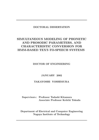
1.2 Proposition of this thesis
The proposed TTS system is shown in Fig. 1.1. This figure shows the training and
synthesis parts of the HMM-based TTS system. In the training phase, first, spectral
parameters (e.g., cepstral coefficients) and excitation parameters (e.g., fundamen-
tal frequency) are extracted from speech database. The extracted parameters are
modeled by context-dependent HMMs. In the systhesis phase, a context-dependent
label sequence is obtained from a input text by text analysis. A sentence HMM is
constructed by concatenating context dependent HMMs according to the context-
dependent label sequence. By using the parameter generation algorithm, spectral
and excitation parameters are generated from the sentence HMM. Finaly, by using
a synthesis filter, speech is synthesized from the generated spectral and excitation
parameters.
In this thesis, it is roughly assumed that spectral and excitation parameters include
phonetic and prosodic information, respectively. If these phonetic and prosodic pa-
rameters are modeled in a unified framework of HMMs, it is possible to apply speaker
adaptation / interpolation techniques to phonetic and prosodic information, simul-
taneously, and synthesize speech with various voice characteristics such as speaker
individualities and emotions. From the point of view, the phonetic and prosodic
parameter modeling technique and the voice conversion technique are proposed in
this thesis.
5
18. Speech signal
SPEECH
DATABASE
Excitation Spectral
parameter parameter
extraction extraction
Excitation parameter Spectral parameter
Training of HMM Training part
Label
Synthesis part
Context dependent
TEXT HMMs
Text analysis
Label Parameter generation
from HMM
Excitation parameter Spectral parameter
Excitation Synthesis SYNTHESIZED
generation filter SPEECH
Figure 1.1: The scheme of the HMM-based TTS system.
The remainder of this thesis is organized as follows:
In Chapters 2–4, the following fundamental techniques of the HMM-based speech
synthesis are described:
• Mel-cepstral analysis and synthesis technique (Chapter 2)
• Speech parameter modeling based on HMM (Chapter 3)
• Speech parameter generation from HMM (Chapter 4)
Chapter 5 presents construction of the proposed HMM-based TTS system in which
spectrum, fundamental frequency (F0), duration are modeled by HMM simultane-
ously, and Chapter 6 discribes how to synthesize speech. In Chapter 7, mixed
excitation model is incorporated into the proposed TTS system in order to improve
6
19. quality of synthesized speech. Chapter 8 presents how to synthesize speech with
various voice characteristics, appling speaker interpolation technique to HMM-based
TTS. Finally Chapter 9 draws overall conclusions and describes possible future
works.
1.3 Original contributions
This thesis describes new approaches to synthesize speech with natural human voice
characteristics and with various voice characteristics such as speaker individuality
and emotion. The major original contributions are as follows:
• Speech parameter generation using multi-mixture HMM.
• Duration modeling for the HMM-based TTS system.
• Simultaneous modeling of spectrum, F0 and duration.
• Training of context dependent HMM using MDL principle.
• F0 parameter generation using dynamic features.
• Automatic training of the HMM-based TTS system.
• Improvement of the quality of the synthesized speech by incorporating the
mixed excitation model and postfilter into the HMM-based TTS system.
• Voice conversion using a speaker interpolation technique.
7
20. Chapter 2
Mel-cepstral Analysis and
Synthesis Technique
The proposed TTS system is based on source-filter model. In order to construct
the system, first, it is necessary to extract feature parameters, which describe the
vocal tract, from speech database for training. For all the work in this thesis, the
mel-cepstral analysis [16] is used for spectral estimation. This chapter describes
the mel-cepstral analysis, how feature parameters, i.e., mel-cepstral coefficients, are
extracted speech signals and how speech is synthesized from the mel-cepstral coef-
ficients.
2.1 Source-filter model
To treat a speech waveform mathematically, source-filter model is generally used
to represent sampled speech signals, as shown in 2.1. The transfer function H(z)
models the structure of vocal tract. The excitation source is chosen by a switch
which controls the voiced/unvoiced character of the speech. The excitation signal
is modeled as either a periodic pulse train for voiced speech, or a random noise
sequence for unvoiced speech. To produce speech signal x(n), the parameters of the
model must change with time. The excitation signal e(n) is filtered by a time-varying
linear system H(z) to generate speech signals x(n).
The speech x(n) can be computed from the excitation e(n) and the impulse response
h(n) of the vocal tract using the convolution sum expression
x(n) = h(n) ∗ e(n) (2.1)
where the symbol ∗ stands for discrete convolution. The details of digital signal
processing and speech processing are given in Ref. [17]
8
21. Fundamental frequency
Vocal Tract
Parameter
Periodic pulse
train
Synthesized
Synthesis Filter
e(n) speech
White noise h(n) x(n) = h(n) ∗ e(n)
Figure 2.1: Source-filter model.
2.2 Mel-cepstral analysis
In mel-cepstral analysis[16], the model spectrum H(ejw ) is represented by the M -th
order mel-cepstral coefficients c(m) as follows:
˜
M
H(z) = exp c(m)˜−m ,
˜ z (2.2)
m=0
where
−1 z −1 − α
z =
˜ , |a| < 1. (2.3)
1 − αz −1
The phase characteristic of the all-pass transfer function z−1 = e−j ω is given by
˜ ˜
(1 − α2 ) sin ω
ω = tan−1
˜ . (2.4)
(1 + α2 ) cos ω − 2α
For example for a sampling frequency of 16kHz, ω is a good approximation to the
˜
mel scale based on subjective pitch evaluations when α = 0.42(Tab. 2.1).
To obtain an unbiased estimate, we use the following criterion [18] and minimize it
with respect to c(m)M
˜ m=0
1 π
E= exp R(ω) − R(ω) − 1dω, (2.5)
2π −π
where
2
R(ω) = log IN (ω) − log H(ejω ) , (2.6)
and IN (ω) is the modified periodogram of a weakly stationary process x(n) with a
time window of length N . To take the gain factor K outside from H(z), we rewrite
Eq.(2.2) as:
M
H(z) = exp b(m)Φm (z) = K · D(z), (2.7)
m=0
9
22. Table 2.1: Examples of α for approximating auditory frequency scales.
Sampling frequency Mel scale Bark scale
8kHz 0.31 0.42
10kHz 0.35 0.47
12kHz 0.37 0.50
16kHz 0.42 0.55
where
K = exp b(0), (2.8)
M
D(z) = exp b(m)Φm (z), (2.9)
m=0
and
c(m) m=M
b(m) = (2.10)
c(m) − αb(m + 1) 0 ≤ m < M
1 m=0
2 −1
Φm (z) = (1 − α )z (2.11)
z −(m−1) m ≥ 1
˜
1 − αz −1
Since H(z) is a minimum phase system, we can show that the minimization of E
with respect to c(m)M is equivalent to that of
˜ m=0
1 π IN (ω)
ε= dω, (2.12)
2π −π |D(ejω )|
with respect to
b = [b(1), b(2), · · · , b(M )]T . (2.13)
∂E
The gain factor K that minimizes E is obtained by setting ∂K
= 0:
√
K= εmin (2.14)
where εmin is the minimized value of ε.
2.3 Synthesis filter
The synthesis filter D(z) of Eq.(2.9) is not a rational function and, therefore, it can-
not be realized directly. Howerver, using Mel Log Spectrum Approximation filter
10
23. Table 2.2: Coefficients of R4 (ω).
l A4,l
1 4.999273 × 10⁻¹
2 1.067005 × 10⁻¹
3 1.170221 × 10⁻²
4 5.656279 × 10⁻⁴
(MLSA filter) [19], the synthesis filter D(z) can be approximated with sufficient ac-
curacy and becomes minimum phase IIR system. The complex exponential function
exp ω is qpproximated by a rational function
exp ω RL (F (z))
L
1+ AL,l ω l
l=1
= L
. (2.15)
1+ AL,l (−ω)l
l=1
Thus D(z) is approximated as follows:
RL (F (z)) exp(F (z)) = D(z) (2.16)
where F (z) is defined by
M
F (z) = b(m)Φm (z). (2.17)
m=1
The filter structure of F (z) is shown in Fig. 2.2(a). Figure 2.2(b) shows the block
diagram of the MLSA filter RL (F (z)) for the case of L = 4.
When we use the coefficients A4,l show in Tab. 2.2, R4 (F (z)) is stable and becomes
a minimum phase system under the condition
|F (ejω )| ≤ 6.2. (2.18)
Further more, we can show that the approximation error | log D(ejω )−log R4 (F (ejω ))|
does not exceed 0.24dB[20] under the condition
|F (ejω )| ≤ 4.5. (2.19)
When F (z) is expressed as
F (z) = F1 (z) + F2 (z) (2.20)
11
24. the exponential transfer function is approximated in a cascade form
D(z) = exp F (z)
= exp F1 (z) · exp F2 (z)
RL (F1 (z)) · RL (F2 (z)) (2.21)
as shown in Fig. 2.2(c). If
max |F1 (ejω )|, max |F2 (ejω )| < max |F (ejω )|, (2.22)
ω ω ω
it is expected that RL (F1 (ejω )) · RL (F2 (ejω )) approximates D(ejω ) more accurately
than RL (F (ejω )).
In the following experiments, we let
F1 (z) = b(1)Φ1 (z) (2.23)
M
F2 (z) = b(m)Φm (z). (2.24)
m=2
Since we empirically found that
max |F1 (ejω )|, max |F2 (ejω )| < 4.5 (2.25)
ω ω
for speech sounds, RL (F1 (z))·RL(F2 (z)) approximates the exponential transfer func-
tion D(z) with sufficient accuracy and becomes a stable system.
12
25. α α α
1 − α2
Input
Z −1 Z −1 Z −1 Z −1
b(1) b(2) b(3)
Output
(a) Basic filter F (z)
Output
Input
F (z) F (z) F (z) F (z)
A4,1 A4,2 A4,3 A4,4
(b) RL (F (z)) D(z), L=4
Input output
R4 (F1 (z)) R4 (F2 (z))
(c) Two stage cascade structure
Figure 2.2: Implementation of Synthesis filter D(z).
13
26. Chapter 3
Speech Parameter Modeling
Based on HMM
The most successful and widely used acoustic models in recent years have been
Hidden Markov Models (HMMs). Practically all major speech recognition systems
are generally implemented using HMM. This chapter describes how to model spectral
and excitation parameters in a framework of HMM.
3.1 Spectral parameter modeling
3.1.1 Continuous density HMM
In this thesis, a continuous density HMM is used for the vocal tract modeling in the
same way as speech recognition systems. The continuous density Markov model is a
finite state machine which makes one state transition at each time unit (i.e, frame).
First, a decision is made to which state to succeed (including the state itself). Then
an output vector is generated according to the probability density function (pdf) for
the current state. An HMM is a doubly stochastic random process, modeling state
transition probabilities between states and output probabilities at each state.
One way of interpreting HMMs is to view each state as a model of a segment of
speech. Figure 3.1 shows an example of representation of a speech utterance using a
N -state left-to-right HMM where each state is modeled by a multi-mixture Gaussian
model. Assume that this utterance(typically parameterized by speech analysis as
the D-dimensional observation vector ot ) is divided into N segments di which are
represented by the states Si . The transition probability aij defines the probability
of moving from state i to state j and satisfies aii + aij = 1. Then, each state can be
14
27. a11 a22 a33 a44 a55
a12 a23 a34 a45
S1 S2 S3 S4 S5 HMM
b1 (ot ) b2 (ot ) b3 (ot ) b4 (ot ) b5 (ot )
Frequency (kHz)
0
2
4 Spectrum
6
8
d1 d2 d3 d4 d5
Figure 3.1: Representation of a speech utterance using a five-state HMM.
modeled by a M -mixtures Gaussian density function:
M
bj (ot ) = cjk N (ot , µjk , Σjk )
k=1
M
1 1
= cjk D
exp − (ot − µjk )T Σ−1 (ot − µjk ) ,
1 jk (3.1)
k=1 (2π) |Σjk |
2 22
where cjk , µjk and Σjk are the mixture coefficient, D-dimensional mean vector and
D × D covariance matrix(full covariance matrix) for the k-th mixture component
in the j-th state, respectively. This covariance can be restricted to the diagonal
elements (diagonal covariance matrix) when the elements of the feature vector are
assumed to be independent. |Σjk | is the determinant of Σjk , and Σ−1 is the inverse
jk
of Σjk . The mixture gains cjk satisfy the stochastic constraint
M
cjk = 1, 1≤j≤N (3.2)
k=1
cjk ≥ 0, 1 ≤ j ≤ N, 1 ≤ k ≤ M (3.3)
15
28. so that the pdf is properly normalized, i.e.,
∞
bj (o)do, 1≤j≤N (3.4)
−∞
Since the pdf of Eq. (3.1) can be used to approximate, arbitrarily closely, any finite,
continuous density function, it can be applied to a wide range of problems and is
widely used for acoustic modeling.
For convenience, to indicate the complete parameter set of the model, we use the
compact notation
λ = (A, B, π), (3.5)
where A = {aij }, B = {bj (o)} and π = {πi }. πi is the initial state distribution of
state i, and it have the property
0, i = 1
π= (3.6)
1, i = 1
in the left-to-right model.
3.1.2 Probability calculation
For calculation of P (O|λ), which is the probability of the observation sequence O =
(o1 , o2 , · · · , oT ) given the model λ, forward-backward algorithm is generally used.
If we calculate P (O|λ) directly without this algorithm, it requires on the order of
2T N 2 calculation. On the other hand, calculation using forward-backward algorithm
requires on the order of N 2 T calculations, and it is computationally feasible. In the
following part, forward-backward algorithm is described.
The forward algorithm
Consider the forward variable αt (i) defined as
αt (i) = P (o1 , o2 , · · · , ot , qt = i|λ) (3.7)
that is, the probability of the partial observation sequence from 1 to t and state i
at time t, given the model λ. We can solve for αt (i) inductively, as follows:
1. Initialization
α1 (i) = πi bi (o1 ), 1 ≤ ileqN. (3.8)
16
29. 2. Induction
N
1≤t≤T −1
αt+1 (j) = αt (i)aij bj (ot+1 ), (3.9)
i=1
1≤j≤N
3. Termination
N
P (O|λ) = αT (i). (3.10)
i=1
The backward algorithm
In the same way as forward algorithm, consider the backward variable βt (i) defined
as
βt (i) = P (ot + 1, ot + 2, · · · , oT |qt = i, λ) (3.11)
that is, the probability of the partial observation sequence from t to T , given state
i at time t and the model λ. We can solve for βt (i) inductively, as follows:
1. Initialization
βT (i) = 1, 1 ≤ i ≤ N. (3.12)
2. Induction
N
t = T − 1, T − 2, · · · , 1
βt (i) = aij bj (ot+1 )βt+1 (j), (3.13)
i=1
1≤i≤N
3. Termination
N
P (O|λ) = β1 (i). (3.14)
i=1
The forward-backward probability calculation is based on the trellis structure shown
in Fig. 3.2. In this figure, the x-axis and y-axis represent observation sequence and
states of Markov model, respectively. On the trellis, all the possible state sequence
will remerge into these N nodes no matter how long the observation sequence. In
the case of the forward algorithm, at times t = 1, we need to calculate values of
α1 (i), 1 ≤ i ≤ N . At times t = 2, 3, · · · , T , we need only calculate values of αt (j),
1 ≤ j ≤ N , where each calculation involves only the N previous values of αt−1 (i)
because each of the N grid points can be reached from only the N grid points at
the previous time slot. As the result, the forward-backward algrorithm can reduce
order of probability calculation.
17
30. N
Si
3
State
2
1
1 2 3 4 T
Observation sequence ot
Figure 3.2: Implementation of the computation using forward-backward algorithm
in terms of a trellis of observation t and state i.
3.1.3 Parameter estimation of continuous density HMM
It is difficult to determine a method to adjust the model parameters (A, B, π) to
satisfy a certain optimization criterion. There is no known way to analytical solve for
the model parameter set that maximizes the probability of the observation sequence
in a closed form. We can, however, choose λ = (A, B, π) such that its likelihood,
P (O|λ), is locally maximized using an iterative procedure such as the Baum-Welch
method(also known as the EM(expectation-maximization method))[21], [22].
To describe the procedure for reestimation of HMM parameters, first, the probability
of being in state i at time t, and state j at time t + 1, given the model and the
observation sequence, is defined as follows:
ξt (i, j) = P (qt = i, qt+1 = j|O, λ), (3.15)
From the definitions of the forward and backward variables, ξt (i, j) is writen in the
form
P (qt = i, qt+1 = j|O, λ)
ξt (i, j) =
P (O|λ)
αt (i)aij bj (ot+1 βt+1 (j))
= N N
(3.16)
αt (i)aij bj (ot+1 βt+1 (j))
i=1 j=1
18
31. Using ξt (i, j), the probability of being in state i at time t, given the entire observation
and the model, is represented by
N
γt (i) = ξt (i, j). (3.17)
j=1
Q-function
The reestimation formulas can be derived directly by maximizing Baum’s auxiliary
funciton
Q(λ , λ) = P (O, q|λ ) log P (O, q|λ) (3.18)
q
over λ. Because
Q(λ , λ) ≥ Q(λ , λ) ⇒ P (O, q|λ ) ≥ P (O, q|λ) (3.19)
We can maximize the function Q(λ , λ) over λ to improve λ in the sense of increasing
the likelihood P (O, q|λ).
Maximization of Q-function
For given observation sequence O and model λ , we derive parameters of λ which
maximize Q(λ , λ). P (O, q|λ) can be written as
T
P (O, q|λ) = πq0 aqt−1 qt bqt (ot ) (3.20)
t=1
T T
log P (O, q|λ) = log πq0 + log aqt−1 qt + log bqt (ot ) (3.21)
t=1 t=1
Hence Q-function (3.18) can be written as
Q(λ , λ) = Qπ (λ , pi)
T
+ Qai (λ , ai )
t=1
T
+ Qbi (λ , bi )
t=1
N
= P (O, q0 = i|λ ) log πi
i=1
N T
+ P (O, qt−1 = i, qt = j|λ ) log aij
j=1 t=1
T
+ P (O, qt = i|λ ) log bi (ot ) (3.22)
t=1
19
32. where
π = [π1 , π2 , · · · , πN ] (3.23)
ai = [ai1 , ai2 , · · · , aiN ] , (3.24)
and bi is the parameter vector that defines bi (·). The parameter set λ which maxi-
mizes (3.22), subject to the stochastic constraints
N
πj = 1, (3.25)
j=1
N
aij = 1, (3.26)
j=1
M
cjk = 1, (3.27)
k=1
∞
bj (o)do = 1, (3.28)
−∞
can be derived as
α0 (i)β0 (i)
πi = N
= γ0 (i) (3.29)
αT (j)
j=1
T T
αt−1 (i)aij bj (ot )βt (j) ξt−1 (i, j)
t=1 t=1
aij = T
= T
(3.30)
αt−1 (i)βt−1 (i) γt−1 (i)
t=1 t=1
The reestimation formulas for the coefficients of the mixture density, i.e, cjk , µjk
and Σjk are of the form
T
γt (j, k)
t=1
cij = T M
(3.31)
γt (j, k)
t=1 k=1
T
γt (j, k) · ot
t=1
µjk = T
(3.32)
γt (j, k)
t=1
T
γt (j, k) · (ot − µjk )(ot − µjk )
t=1
Σjk = T
(3.33)
γt (j, k)
t=1
20
33. voiced region (continuous value)
200
Frequency (Hz)
150
100
50
0 1 2 3 4 5
time (s)
unvoiced region (discrete symbol)
Figure 3.3: Example of F0 pattern.
(3.34)
where γt (j, k) is the probability of being in state j at time t with the kth mixture
component accounting for ot , i.e.,
α (j)β (j) c N (o , µ , Σ )
t t jk t jk jk
γt (j, k) = N M . (3.35)
αt (j)βt (j) N (ot , µjk , Σjk )
j=1 m=1
3.2 F0 parameter modeling
The F0 pattern is composed of continuous values in the “voiced” region and a
discrete symbol in the “unvoiced” region (Fig.3.3). Therefore, it is difficult to apply
the discrete or continuous HMMs to F0 pattern modeling. Several methods have
been investigated [23] for handling the unvoiced region: (i) replacing each “unvoiced”
symbol by a random vector generated from a probability density function (pdf) with
a large variance and then modeling the random vectors explicitly in the continuous
HMMs [24], (ii) modeling the “unvoiced” symbols explicitly in the continuous HMMs
by replacing “unvoiced” symbol by 0 and adding an extra pdf for the “unvoiced”
symbol to each mixture, (iii) assuming that F0 values is always exist but they cannot
observed in the unvoiced region and applying the EM algorithm [25]. In this section,
A kind of HMM for F0 pattern modeling, in which the state output probabilities
are defined by multi-space probability distributions (MSDs), is described.
21
34. 3.2.1 Multi-Space Probability Distribution
We consider a sample space Ω shown in Fig. 3.4, which consists of G spaces:
G
Ω= Ωg (3.36)
g=1
where Ωg is an ng -dimensional real space Rng , and specified by space index g. Each
space Ωg has its probability wg , i.e., P (Ωg ) = wg , where G wg = 1. If ng > 0, each
g=1
space has a probability density function Ng (x), x ∈ Rng , where Rng Ng (x)dx = 1.
We assume that Ωg contains only one sample point if ng = 0. Accordingly, letting
P (E) be the probability distribution, we have
G G
P (Ω) = P (Ωg ) = wg Ng (x)dx = 1. (3.37)
g=1 g=1 Rng
It is noted that, although Ng (x) does not exist for ng = 0 since Ωg contains only
one sample point, for simplicity of notation, we define as Ng (x) ≡ 1 for ng = 0.
Each event E, which will be considered in this thesis, is represented by a random
variable o which consists of a continuous random variable x ∈ Rn and a set of space
indices X, that is,
o = (x, X) (3.38)
where all spaces specified by X are n-dimensional. The observation probability of
o is defined by
b(o) = wg Ng (V (o)) (3.39)
g∈S(o)
where
V (o) = x, S(o) = X. (3.40)
Some examples of observations are shown in Fig. 3.4. An observation o1 consists of
three-dimensional vector x1 ∈ R3 and a set of space indices X1 = {1, 2, G}. Thus
the random variable x is drawn from one of three spaces Ω1 , Ω2 , ΩG ∈ R3 , and its
probability density function is given by w1 N1 (x) + w2 N2 (x) + wG NG (x).
The probability distribution defined in the above, which will be referred to as multi-
space probability distribution (MSD) in this thesis, is the same as the discrete distri-
bution and the continuous distribution when ng ≡ 0 and ng ≡ m > 0, respectively.
Further, if S(o) ≡ {1, 2, . . . , G}, the continuous distribution is represented by a
G-mixture probability density function. Thus multi-space probability distribution
is more general than either discrete or continuous distributions.
22
35. Sample Space Ω
Space
Index Space pdf of x Observation
Ω1 = R3
1 w1 o1 = ( x1, {1, 2, G})
N1 ( x ) x1 ∈ R3
Ω 2 = R3
2 w2
N2 ( x ) o2 = ( x2 , {1, G})
x2 ∈ R3
Ω 3 = R5
3 w3
N3 ( x )
o3 = ( x3 , {3})
x3 ∈ R 5
Ω G = R3 wG
G
NG ( x )
Figure 3.4: Multi-space probability distribution and observations.
3.2.2 Multi-space distribution HMM
The output probability in each state of MSD-HMM is given by the multi-space
probability distribution defined in the previous section. An N -state MSD-HMM λ
is specified by initial state probability distribution π = {πj }N , the state transition
j=1
probability distribution A = {aij }Nj=1 , and state output probability distribution
i,
B = {bi (·)}N , where
i=1
bi (o) = wig Nig (V (o)), i = 1, 2, . . . , N. (3.41)
g∈S(o)
As shown in Fig. 3.5, each state i has G probability density functions Ni1 (·), Ni2 (·),
. . ., NiG (·), and their weights wi1 , wi2 , . . ., wiG .
23
36. 1 2 3
w11 w21 w31
Ω1 = R n1
N11 ( x ) N21 ( x ) N31 ( x )
w12 w22 w32
Ω 2 = Rn2
N12 ( x ) N22 ( x ) N32 ( x )
w1G w2 G w3G
Ω G = RnG
N1G ( x ) N2 G ( x ) N3 G ( x )
Figure 3.5: An HMM based on multi-space probability distribution.
Observation probability of O = {o1 , o2 , . . . , oT } is written as
T
P (O|λ) = aqt−1 qt bqt (ot )
all q t=1
T
= aqt−1 qt wqt lt Nqt lt (V (ot )) (3.42)
all q,l t=1
where q = {q1 , q2 , . . . , qT } is a possible state sequence, l = {l1 , l2 , . . . , lT } ∈ {S(o1 )×
S(o2 )×. . .×S(oT )} is a sequence of space indices which is possible for the observation
sequence O, and aq0 j denotes πj .
The forward and backward variables:
αt (i) = P (o1 , o2 , . . . , ot , qt = i|λ) (3.43)
βt (i) = P (ot+1 , ot+2 , . . . , oT |qt = i, λ) (3.44)
can be calculated with the forward-backward inductive procedure in a manner simi-
lar to the conventional HMMs. According to the definitions, (3.42) can be calculated
as
N N
P (O|λ) = αT (i) = β1 (i). (3.45)
i=1 i=1
24
37. The forward and backward variables are also used for calculating the reestimation
formulas derived in the the next section
3.2.3 Reestimation algorithm for MSD-HMM training
For a given observation sequence O and a particular choice of MSD-HMM, the ob-
jective in maximum likelihood estimation is to maximize the observation likelihood
P (O|λ) given by (3.42), over all parameters in λ. In a manner similar to [21], [22], we
derive reestimation formulas for the maximum likelihood estimation of MSD-HMM.
Q-function
An auxiliary function Q(λ , λ) of current parameters λ and new parameter λ is
defined as follows:
Q(λ , λ) = P (O, q, l|λ ) log P (O, q, l|λ) (3.46)
all q,l
In the following, we assume Nig (·) to be the Gaussian density with mean vector µig
and covariance matrix Σig .
Theorem 1
Q(λ , λ) ≥ Q(λ , λ ) → P (O, λ) ≥ P (O, λ )
Theorem 2 If, for each space Ωg , there are among V (o1 ), V (o2 ), . . ., V (oT ), ng +1
observations g ∈ S(ot ), any ng of which are linearly independent, Q(λ , λ) has a
unique global maximum as a function of λ, and this maximum is the one and only
critical point.
Theorem 3 A parameter set λ is a critical point of the likelihood P (O|λ) if and
only if it is a critical point of the Q-function.
We define the parameter reestimates to be those which maximize Q(λ , λ) as a
function of λ, λ being the latest estimates. Because of the above theorems, the
sequence of resetimates obtained in this way produce a monotonic increase in the
likelihood unless λ is a critical point of the likelihood.
25
38. Maximization of Q-function
For given observation sequence O and model λ , we derive parameters of λ which
maximize Q(λ , λ). From (3.42), log P (O, q, l|λ) can be written as
log P (O, q, l|λ)
T
= log aqt−1 qt + log wqt lt + log Nqt lt (V (ot )) . (3.47)
t=1
Hence Q-function (3.46) can be written as
N
Q(λ , λ) = P (O, q1 = i|λ ) log πi
i=1
N T −1
+ P (O, qt = i, qt+1 = j|λ ) log aij
i,j=1 t=1
N G
+ P (O, qt = i, lt = g|λ ) log wig
i=1 g=1 t∈T (O,g)
N G
+ P (O, qt = i, lt = g|λ ) log Nig (V (ot ))
i=1 g=1 t∈T (O,g)
(3.48)
where
T (O, g) = {t | g ∈ S(ot )}. (3.49)
The parameter set λ = (π, A, B) which maximizes (3.48), subject to the stochastic
constraints N πi = 1, N aij = 1 and G wg = 1, can be derived as
i=1 j=1 g=1
πi = γ1 (i, g) (3.50)
g∈S(o1 )
T −1
ξt (i, j)
t=1
aij = T −1
(3.51)
γt (i, g)
t=1 g∈S(ot )
γt (i, g)
t∈T (O,g)
wig = G
(3.52)
γt (i, h)
h=1 t∈T (O,h)
γt (i, g) V (ot )
t∈T (O,g)
µig = , ng > 0 (3.53)
γt (i, g)
t∈T (O,g)
26
39. γt (i, g)(V (ot ) − µig )(V (ot ) − µig )T
t∈T (O,g)
Σig = ,
γt (i, g)
t∈T (O,g)
ng > 0 (3.54)
where γt (i, h) and ξt (i, j) can be calculated by using the forward variable αt (i) and
backward variable βt (i) as follows:
γt (i, h) = P (qt = i, lt = h|O, λ)
αt (i)βt (i) wih Nih (V (ot ))
= N · (3.55)
wig Nig (V (ot ))
αt (j)βt (j) g∈S(ot )
j=1
ξt (i, j) = P (qt = i, qt+1 = j|O, λ)
αt (i)aij bj (ot+1 )βt+1 (j)
= N N (3.56)
αt (h)ahk bk (ot+1 )βt+1 (k)
h=1 k=1
From the condition mentioned in Theorem 2, it can be shown that each Σig is
positive definite.
3.2.4 Application to F0 pattern modeling
The MSD-HMM includes the discrete HMM and the continuous mixture HMM
as special cases since the multi-space probability distribution includes the discrete
distribution and the continuous distribution. If ng ≡ 0, the MSD-HMM is the same
as the discrete HMM. In the case where S(ot ) specifies one space, i.e., |S(ot )| ≡ 1,
the MSD-HMM is exactly the same as the conventional discrete HMM. If |S(ot )| ≥ 1,
the MSD-HMM is the same as the discrete HMM based on the multi-labeling VQ
[26]. If ng ≡ m > 0 and S(o) ≡ {1, 2, . . . , G}, the MSD-HMM is the same as
the continuous G-mixture HMM. These can also be confirmed by the fact that if
ng ≡ 0 and |S(ot )| ≡ 1, the reestimation formulas (3.50)-(3.52) are the same as those
for discrete HMM of codebook size G, and if ng ≡ m and S(ot ) ≡ {1, 2, . . . , G},
the reestimation formulas (3.50)-(3.54) are the same as those for continuous HMM
with m-dimensional G-mixture densities. Further, the MSD-HMM can model the
sequence of observation vectors with variable dimension including zero-dimensional
observations, i.e., discrete symbols.
While the observation of F0 has a continuous value in the voiced region, there exist
no value for the unvoiced region. We can model this kind of observation sequence
assuming that the observed F0 value occurs from one-dimensional spaces and the
27
40. “unvoiced” symbol occurs from the zero-dimensional space defined in Section 3.2.1,
that is, by setting ng = 1 (g = 1, 2, . . . , G − 1), nG = 0 and
{1, 2, . . . , G − 1}, (voiced)
S(ot ) = , (3.57)
{G}, (unvoiced)
the MSD-HMM can cope with F0 patterns including the unvoiced region without
heuristic assumption. In this case, the observed F0 value is assumed to be drawn
from a continuous (G − 1)-mixture probability density function.
28
41. Chapter 4
Speech parameter generation from
HMM
The performance of speech recognition based on HMMs has been improved by incor-
porating the dynamic features of speech. Thus we surmise that, if there is a method
for speech parameter generation from HMMs which include the dynamic features, it
will be useful for speech synthesis by rule. This chapter derives a speech parameter
generation algorithm from HMMs which include the dynamic features.
4.1 Speech parameter generation based on maxi-
mum likelihood criterion
For a given continuous mixture HMM λ, we derive an algorithm for determining
speech parameter vector sequence
O = o1 , o2 , . . . , oT (4.1)
in such a way that
P (O|λ) = P (O, Q|λ) (4.2)
all Q
is maximized with respect to O, where
Q = {(q1 , i1 ), (q2 , i2 ), . . . , (qT , iT )} (4.3)
is the state and mixture sequence, i.e., (q, i) indicates the i-th mixture of state
q. We assume that the speech parameter vector ot consists of the static feature
vector ct = [ct (1), ct (2), . . . , ct (M )] (e.g., cepstral coefficients) and dynamic feature
29
42. vectors ∆ct , ∆2 ct (e.g., delta and delta-delta cepstral coefficients, respectively), that
is, ot = [ct , ∆ct , ∆2 ct ] , where the dynamic feature vectors are calculated by
(1)
L+
∆ct = w (1) (τ )ct+τ (4.4)
(1)
τ =−L−
(2)
L+
∆2 ct = w (2) (τ )ct+τ . (4.5)
(2)
τ =−L−
We have derived algorithms [11], [12] for solving the following problems:
Case 1. For given λ and Q, maximize P (O|Q, λ) with respect to O under the
conditions (4.4), (4.5).
Case 2. For a given λ, maximize P (O, Q|λ) with respect to Q and O under the
conditions (4.4), (4.5).
In this section, we will review the above algorithms and derive an algorithm for the
problem:
Case 3. For a given λ, maximize P (O|λ) with respect to O under the conditions
(4.4), (4.5).
4.1.1 Case 1: Maximizing P (O|Q, λ) with respect to O
First, consider maximizing P (O|Q, λ) with respect to O for a fixed state and mixture
sequence Q. The logarithm of P (O|Q, λ) can be written as
1
log P (O|Q, λ) = − O U −1 O + O U −1 M + K (4.6)
2
where
U −1 = diag U −1 1 , U −1 2 , ..., U −1,iT
q1 ,i q2 ,i qT (4.7)
M = µq1 ,i1 , µq2 ,i2 , ..., µqT ,iT (4.8)
µqt , it and U qt , it are the 3M × 1 mean vector and the 3M × 3M covariance ma-
trix, respectively, associated with it -th mixture of state qt , and the constant K is
independent of O.
30
43. It is obvious that P (O|Q, λ) is maximized when O = M without the conditions
(4.4), (4.5), that is, the speech parameter vector sequence becomes a sequence of
the mean vectors. Conditions (4.4), (4.5) can be arranged in a matrix form:
O = WC (4.9)
where
C = [c1 , c2 , . . . , cT ] (4.10)
W = [w 1 , w2 , . . . , wT ] (4.11)
(0) (1) (2)
wt = wt , wt , wt (4.12)
(n) (n)
wt = [ 0M ×M , . . . , 0M ×M , w (n) (−L− )I M ×M ,
1st (n)
(t−L− )-th
(n)
. . . , w(n) (0)I M ×M , . . . , w(n) (L+ )I M ×M ,
t-th (n)
(t+L+ )-th
0M ×M , . . . , 0M ×M ] , n = 0, 1, 2 (4.13)
T -th
(0) (0)
L− = L+ = 0, and w (0) (0) = 1. Under the condition (4.9), maximizing P (O|Q, λ)
with respect to O is equivalent to that with respect to C. By setting
∂ log P (W C|Q, λ)
= 0, (4.14)
∂C
we obtain a set of equations
W U −1 W C = W U −1 M . (4.15)
For direct solution of (4.15), we need O(T 3M 3 ) operations1 because W U −1 W is a
T M × T M matrix. By utilizing the special structure of W U −1 W , (4.15) can be
solved by the Cholesky decomposition or the QR decomposition with O(T M3 L2 )
operations2 , where L = maxn∈{1,2},s∈{−,+} L(n) . Equation (4.15) can also be solved
s
by an algorithm derived in [11], [12], which can operate in a time-recursive manner
[28].
4.1.2 Case 2: Maximizing P (O, Q|λ) with respect to O and
Q
This problem can be solved by evaluating max P (O, Q|λ) = max P (O|Q, λ)P (Q|λ)
for all Q. However, it is impractical because there are too many combinations of
1
When U q,i is diagonal, it is reduced to O(T 3 M ) since each of the M -dimensions can be
calculated independently.
2 (1) (1)
When U q,i is diagonal, it is reduced to O(T M L 2 ). Furthermore, when L− = −1, L+ = 0,
and w(2) (i) ≡ 0, it is reduced to O(T M ) as described in [27].
31
44. Q. We have developed a fast algorithm for searching for the optimal or sub-optimal
state sequence keeping C optimal in the sense that P (O|Q, λ) is maximized with
respect to C [11], [12].
To control temporal structure of speech parameter sequence appropriately, HMMs
should incorporate state duration densities. The probability P (O, Q|λ) can be writ-
ten as P (O, Q|λ) =
P (O, i|q, λ)P (q|λ), where q = {q1 , q2 , . . . , qT }, i = {i1 , i2 ,
. . . , iT }, and the state duration probability P (q|λ) is given by
N
log P (q|λ) = log pqn (dqn ) (4.16)
n=1
where the total number of states which have been visited during T frames is N , and
pqn (dqn ) is the probability of dqn consecutive observations in state qn . If we determine
the state sequence q only by P (q|λ) independently of O, maximizing P (O, Q|λ) =
P (O, i|q, λ)P (q|λ) with respect to O and Q is equivalent to maximizing P (O, i|q, λ)
with respect to O and i. Furthermore, if we assume that state output probabilities
are single-Gaussian, i is unique. Therefore, the solution is obtained by solving (4.15)
in the same way as the Case 1.
4.1.3 Case 3: Maximizing P (O|λ) with respect to O
We derive an algorithm based on an EM algorithm, which find a critical point of
the likelihood function P (O|λ). An auxiliary function of current parameter vector
sequence O and new parameter vector sequence O is defined by
Q(O, O ) = P (O, Q|λ) log P (O , Q|λ). (4.17)
all Q
It can be shown that by substituting O which maximizes Q(O, O ) for O, the
likelihood increases unless O is a critical point of the likelihood. Equation (4.17)
can be written as
1
Q(O, O ) = P (O|λ) − O U −1 O + O U −1 M + K (4.18)
2
where
U −1 = diag U −1 , U −1 , . . . , U −1
1 2 T (4.19)
U −1 =
t γt (q, i)U −1
q,i (4.20)
q,i
U −1 M = U −1 µ1 , U −1 µ2 , . . . , U −1 µT
1 2 T (4.21)
U −1 µt =
t γt (q, i) U −1 µq,i
q,i (4.22)
q,i
32
45. and the constant K is independent of O . The occupancy probability γt (q, i) defined
by
γt (q, i) = P (qt = (q, i)|O, λ) (4.23)
can be calculated with the forward-backward inductive procedure. Under the con-
dition O = W C , C which maximizes Q(O, O ) is given by the following set of
equations:
W U −1 W C = W U −1 M . (4.24)
The above set of equations has the same form as (4.15). Accordingly, it can be
solved by the algorithm for solving (4.15).
The whole procedure is summarized as follows:
Step 0. Choose an initial parameter vector sequence C.
Step 1. Calculate γt (q, i) with the forward-backward algorithm.
Step 2. Calculate U −1 and U −1 M by (4.19)–(4.22), and solve (4.24).
Step 3. Set C = C . If a certain convergence condition is satisfied, stop; otherwise,
goto Step 1.
From the same reason as Case 2, HMMs should incorporate state duration densi-
ties. If we determine the state sequence q only by P (q|λ) independently of O in a
manner similar to the previous section, only the mixture sequence i is assumed to
be unobservable3 . Further, we can also assume that Q is unobservable but phoneme
or syllable durations are given.
4.2 Example
A simple experiment of speech synthesis was carried out using the parameter gener-
ation algorithm. We used phonetically balanced 450 sentences from ATR Japanese
speech database for training. The type of HMM used was a continuous Gaussian
model. The diagonal covariances were used. All models were 5-state left-to-right
models with no skips. The heuristic duration densities were calculated after the
training. Feature vector consists of 25 mel-cepstral coefficients including the zeroth
coefficient, their delta and delta-delta coefficients. Mel-cepstral coefficients were ob-
tained by the mel-cepstral analysis. The signal was windowed by a 25ms Black man
window with a 5ms shift.
3
For this problem, an algorithm based on a direct search has also been proposed in [29].
33
46. Frequency (kHz)
0
2
4
6
8
(a) without dynamic features
Frequency (kHz)
0
2
4
6
8
(b) with delta parameters
Frequency (kHz)
0
2
4
6
8
(c) with delta and delta-delta parameters
Figure 4.1: Spectra generated with dynamic features for a Japanese phrase “chi-
isanaunagi”.
4.2.1 Effect of dynamic feature
First, we observed the parameter generation in the case 1, in which parameter
sequence O maximizes P (O|Q, λ). State sequence Q was estimated from the re-
sult of Veterbi alignment of natural speech. Fig. 4.1 shows the spectra calculated
from the mel-cepstral coefficients generated by the HMM, which is composed by
concatenation of phoneme models. Without the dynamic features, the parame-
ter sequence which maximizes P (O|Q, λ) becomes a sequence of the mean vectors
(Fig. 4.1(a)). On the other hand, Fig. 4.1(b) and Fig. 4.1(c) show that appropriate
parameter sequences are generated by using the static and dynamic feature. Look-
ing at Fig. 4.1(b) and Fig. 4.1(c) closely, we can see that incorporation of delta-delta
parameter improves smoothness of generated speech spectra.
Fig 4.2 shows probability density functions and generated parameters for the zero-th
mel-cepstral coefficients. The x-axis represents frame number. A gray box and its
middle line represent standard deviation and mean of probability density function,
respectively, and a curved line is the generated zero-th mel-cepstral coefficients.
From this figure, it can be observed that parameters are generated taking account
of constraints of their probability density function and dynamic features.
34
47. 7.2
c(0)
4.9
0.38
∆c(0)
-0.31
∆2 c(0)
0.070
-0.068
frame
standard deviation generated parameter
mean
Figure 4.2: Relation between probability density function and generated parameter
for a Japanese phrase “unagi” (top: static, middle: delta, bottom: delta-delta).
35
48. 4.2.2 Parameter generation using multi-mixuture HMM
In the algorithm of the case 3, we assumed that the state sequence (state and mixture
sequence for the multi-mixture case) or a part of the state sequence is unobservable
(i.e., hidden or latent). As a result, the algorithm iterates the forward-backward
algorithm and the parameter generation algorithm for the case where state sequence
is given. Experimental results show that by using the algorithm, we can reproduce
clear formant structure from multi-mixture HMMs as compared with that produced
from single-mixture HMMs.
It has found that a few iterations are sufficient for convergence of the proposed
algorithm. Fig. 4.3 shows generated spectra for a Japanese sentence fragment “kiN-
zokuhiroo” taken from a sentence which is not included in the training data. Fig. 4.4
compares two spectra obtained from single-mixure HMMs and 8-mixture HMMs, re-
spectively, for the same temporal position of the sentence fragment. It is seen from
Fig. 4.3 and Fig. 4.4 that with increasing mixtures, the formant structure of the
generated spectra get clearer.
We evaluated two synthesized speech obtained from single-mixure HMMs and 8-
mixture HMMs by listening test, where fundamental frequency and duration is ob-
tained from natural speech. Figure 4.5 shows the result of pair comparison test.
From the listening test, it has been observed that the quality of the synthetic speech
is considerably improved by increasing mixtures.
When we use single-mixture HMMs, the formant structure of spectrum correspond-
ing to each mean vector µq,i might be vague since µq,i is the average of different
speech spectra. One can increase the number of decision tree leaf clusters. However,
it might result in perceivable discontinuities in synthetic speech since overly large
tree will be overspecialized to training data and generalized poorly. We expect that
the proposed algorithm can avoid this situation in a simple manner.
36
50. 1-mixture 40.8
8-mixtures 59.2
0 20 40 60 80 100
Preference score (%)
Figure 4.5: The result of the pair comparison test.
38
51. Chapter 5
Construction of HMM-based
Text-to-Speech System
Phonetic parameter and prosodic parameter are modeled simultaneously in a unified
framework of HMM. In the proposed system, mel-cepstrum, fundamental frequency
(F0) and state duration are modeled by continuous density HMMs, multi-space
probability distribution HMMs and multi-dimensional Gaussian distributions, re-
spectively. The distributions for spectrum, F0, and the state duration are clustered
independently by using a decision-tree based context clustering technique. This
chapter describes feature vector modeled by HMM, structure of HMM and how to
train context-dependent HMM.
5.1 Calculation of dynamic feature
In this thesis, mel-cepstral coefficient is used as spectral parameter. Mel-cepstral
coefficient vectors c are obtained from speech database using a mel-cepstral analysis
technique [16]. Their dynamic feature ∆c and ∆2 c are calculated as follows:
1 1
∆ct = − ct−1 + ct+1 , (5.1)
2 2
2 1 1 1
∆ ct = ct−1 − ct + ct+1 . (5.2)
4 2 4
In the same way, dynamic features for F0 are calculated by
1 1
δpt = − pt−1 + pt+1 , (5.3)
2 2
1 1 1
δ 2 pt = pt−1 − pt + pt+1 . (5.4)
4 2 4
39
52. represents a continous value ( voiced ).
represents a discrete symbol ( unvoiced ).
Unvoiced region Voiced region Unvoiced region
Delta-delta δ 2 pt
Delta δpt
Static pt−1 pt pt+1
1 t T
Frame number
Figure 5.1: Calculation of dynamic features for F0.
where, in unvoiced region, pt , δpt and δ 2 pt are defined as a discrete symbol. When
dynamic features at the boundary between voiced and unvoiced can not be calcu-
lated, they are defined as a discrete symbol. For example, if dynamic features are
p
calculated by Eq.(5.3)(5.4), δpt and δt at the boundary between voiced and unvoiced
as shown Fig. 5.1 become discrete symbol.
5.2 Spectrum and F0 modeling
In the chapter 3, it is described that sequence of mel-cepstral coefficient vector and
F0 pattern are modeled by a continuous density HMM and multi-space probability
distribution HMM, respectively.
We construct spectrum and F0 models by using embedded training because the
embedded training does not need label boundaries when appropriate initial models
are available. However, if spectrum models and F0 models are embedded-trained
separately, speech segmentations may be discrepant between them.
To avoid this problem, context dependent HMMs are trained with feature vector
which consists of spectrum, F0 and their dynamic features (Fig. 5.2). As a result,
HMM has four streams as shown in Fig. 5.3.
40
53. c
Stream 1
∆c Continuous probability distribution
(Spectrum part)
2
∆ c
p Multi−space probability distribution
Stream 2
δp Multi−space probability distribution
(F0 part) 2
δ p Multi−space probability distribution
Figure 5.2: Feature vector.
Mel-cepstrum N-dimensional
Gaussian
distribution
Voiced
Unvoiced 1-dimensional
Gaussian
Voiced distribution
F0
Unvoiced 0-dimensional
Gaussian
Voiced distribution
Unvoiced
Figure 5.3: structure of HMM.
41
54. 5.3 Duration modeling
5.3.1 Overview
There have been proposed techniques for training HMMs and their state duration
densities simultaneously (e.g., [30]). However, these techniques require a large stor-
age and computational load. In this thesis, state duration densities are estimated
by using state occupancy probabilities which are obtained in the last iteration of
embedded re-estimation [31].
In the HMM-based speech synthesis system described above, state duration densities
were modeled by single Gaussian distributions estimated from histograms of state
durations which were obtained by the Viterbi segmentation of training data. In this
procedure, however, it is impossible to obtain variances of distributions for phonemes
which appear only once in the training data.
In this thesis, to overcome this problem, Gaussian distributions of state durations
are calculated on the trellis(Section 3.1.2) which is made in the embedded training
stage. State durations of each phoneme HMM are regarded as a multi-dimensional
observation, and the set of state durations of each phoneme HMM is modeled by
a multi-dimensional Gaussian distribution. Dimension of state duration densities is
equal to number of state of HMMs, and nth dimension of state duration densities
is corresponding to nth state of HMMs1 . Since state durations are modeled by
continuous distributions, our approach has the following advantages:
• The speaking rate of synthetic speech can be varied easily.
• There is no need for label boundaries when appropriate initial models are
available since the state duration densities are estimated in the embedded
training stage of phoneme HMMs.
In the following sections, we describe training and clustering of state duration mod-
els, and determination of state duration in the synthesis part.
5.3.2 Training of state duration models
There have been proposed techniques for training HMMs and their state duration
densities simultaneously, however, these techniques is inefficient because it requires
huge storage and computational load. From this point of view, we adopt another
technique for training state duration models.
1
We assume the left-to-right model with no skip.
42
55. State duration densities are estimated on the trellis which is obtained in the em-
bedded training stage. The mean ξ(i) and the variance σ2 (i) of duration density of
state i are determined by
T T
χt0 ,t1 (i)(t1 − t0 + 1)
t0 =1 t1 =t0
ξ(i) = T T
, (5.5)
χt0 ,t1 (i)
t0 =1 t1 =t0
T T
χt0 ,t1 (i)(t1 − t0 + 1)2
t0 =1 t1 =t0
σ 2 (i) = T T
− ξ 2 (i), (5.6)
χt0 ,t1 (i)
t0 =1 t1 =t0
respectively, where χt0 ,t1 (i) is the probability of occupying state i from time t0 to t1
and can be written as
t1
χt0 ,t1 (i) = (1 − γt0 −1 (i)) · γt (i) · (1 − γt1 +1 (i)), (5.7)
t=t0
where γt (i) is the occupation probability of state i at time t, and we define γ−1 (i) =
γT +1(i) = 0.
5.4 Context dependent model
5.4.1 Contextual factors
There are many contextual factors (e.g., phone identity factors, stress-related factors,
locational factors) that affect spectrum, F0 and duration. In this thesis, following
contextual factors are taken into account:
• mora2 count of sentence
• position of breath group in sentence
• mora count of {preceding, current, succeeding} breath group
• position of current accentual phrase in current breath group
• mora count and accent type of {preceding, current, succeeding} accentual
phrase
2
A mora is a syllable-sized unit in Japanese.
43
56. • {preceding, current, succeeding} part-of-speech
• position of current phoneme in current accentual phrase
• {preceding, current, succeeding} phoneme
Note that a context dependent HMM corresponds to a phoneme.
5.4.2 Decision-tree based context clustering
When we construct context dependent models taking account of many combina-
tions of the above contextual factors, we expect to be able to obtain appropriate
models. However, as contextual factors increase, their combinations also increase
exponentially. Therefore, model parameters with sufficient accuracy cannot be esti-
mated with limited training data. Furthermore, it is impossible to prepare speech
database which includes all combinations of contextual factors.
Introduction of context clustering
To overcome the above problem, we apply a decision-tree based context clustering
technique [32] to distributions for spectrum, F0 and state duration.
The decision-tree based context clustering algorithm have been extended for MSD-
HMMs in [33]. Since each of spectrum, F0 and duration have its own influential
contextual factors, the distributions for spectral parameter and F0 parameter and
the state duration are clustered independently (Fig. 5.4.2).
Example of decision tree
We used phonetically balanced 450 sentences from ATR Japanese speech database
for training. Speech signals were sampled at 16 kHz and windowed by a 25-ms
Blackman window with a 5-ms shift, and then mel-cepstral coefficients were obtained
by the mel-cepstral analysis3 . Feature vector consists of spectral and F0 parameter
vectors. Spectral parameter vector consists of 25 mel-cepstral coefficients including
the zeroth coefficient, their delta and delta-delta coefficients. F0 parameter vector
consists of log F0, its delta and delta-delta. We used 3-state left-to-right HMMs
with single diagonal Gaussian output distributions. Decision trees for spectrum, F0
and duration models were constructed as shown in Fig. 5.4.2. The resultant trees
3
The source codes of the mel-cepstral analysis/synthesis can be found in
http://kt−lab.ics.nitech.ac.jp/˜tokuda/SPTK/ .
44
57. State Duration
Model
HMM
for Spectrum S1 S2 S3
and F0
Decision Tree Decision Tree
for for
Spectrum State Duration Model
Decision Tree
for
F0
Figure 5.4: Decision trees.
45