Cara Menggugurkan Sperma Yang Masuk Rahim Biyar Tidak Hamil
3.pdf
1. Unit:
Curve-Fitting
Introduction:
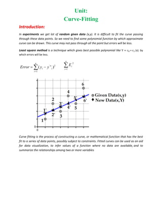
In experiments we get lot of random given data (x,y). It is difficult to fit the curve passing
through these data points. So we need to find some polynomial function by which approximate
curve can be drawn. This curve may not pass through all the point but errors will be less.
Least square method is a technique which gives best possible polynomial like Y c + c (x). by
which errors will be less.
' 2
1
( )
n
n
i i
i
Error y y
n
i
i
E
1
2
Curve fitting is the process of constructing a curve, or mathematical function that has the best
fit to a series of data points, possibly subject to constraints. Fitted curves can be used as an aid
for data visualization, to infer values of a function where no data are available, and to
summarize the relationships among two or more variables
2. A first degree polynomial equation:
Yn c + c (x).
A first degree polynomial equation is
an exact fit through any two points
with distinct x coordinates.
A second degree polynomial: Yn c + c (x) + c (x)2
.
Fitting a Line (first degree polynomial) equation:
n= number of data points
∑
∑ ∑
∑ .
∑
OR
Determinants:
d=det d1= d2=
Constants: c0=d1/d & c1=d2/d
Fitting a Line : + (x).
Problem: Using least square method Fit a line: Yn c + c (x)
X 1 2 3 4
Y 2 6 12 20
Solution: n= number of data points=4
∑
∑ ∑
∑ .
∑
X Y
1 2 1 2
2 3 4 12
3 12 9 36
4 20 16 80
∑ =10 ∑ .
40 ∑ 30 ∑ 130
5. Solved Problems
Fit the line yn=c0+c1*x
x=[1 2 3 4];
y=[2 6 12 20];
‐‐‐‐‐‐‐‐‐‐‐‐‐‐‐‐‐
X Y X2
XY
‐‐‐‐‐‐‐‐‐‐‐‐‐‐‐‐‐
1 2 1 2
2 6 4 12
3 12 9 36
4 20 16 80
‐‐‐‐‐‐‐‐‐‐‐‐‐‐‐‐‐
10 40 30 130
Calculate d d1 d2 c 0 c1 by you
BEST FIT ,Yn=‐5.000+6.000(X)
Fit the line yn=c0+c1*x
L=a0+a1T
x=[ 20 30 40 50 60 70];
y=[800.3 800.4 800.6 800.7 800.9 801];
‐‐‐‐‐‐‐‐‐‐‐‐‐‐‐‐‐‐‐‐‐‐‐
X Y X2
X.*Y
‐‐‐‐‐‐‐‐‐‐‐‐‐‐‐‐‐‐‐‐‐‐‐
20 800 400 16006
30 800 900 24012
40 801 1600 32024
50 801 2500 40035
60 801 3600 48054
70 801 4900 56070
‐‐‐‐‐‐‐‐‐‐‐‐‐‐‐‐‐‐‐‐‐‐‐‐‐‐‐‐‐
270 4804 13900 216201
‐‐‐‐‐‐‐‐‐‐‐‐‐‐‐‐‐‐‐‐‐‐‐‐‐‐‐‐‐
Calculate d d1 d2 c 0 c1 by you
6. BEST FIT ,Yn=799.994+0.015(X)
Fitting a second degree polynomial:
+ (X) + (X)2
∑ ∑
∑ ∑ ∑
∑ ∑ ∑
0
1
2
∑
∑
∑
.
1 2
1 2 3
2 3 4
0
1
2
5
6
7
D det
1 2
1 2 3
2 3 4
D1 det
5 1 2
6 2 3
7 3 4
D2 Det
5 2
1 6 3
2 7 4
D3 Det
1 5
1 2 6
2 3 7
Constants: C0=d1/d , C1=d2/d and C2=d3/d
Problem: Using least square method fit a second degree polynomial
+ (X) + (X)2
X 1 2 3 4 5 6 7 8 9
Y 2 6 7 8 10 11 11 10 9
Solution:
∑ ∑
∑ ∑ ∑
∑ ∑ ∑
∑
∑
∑
=
0
1
2
7. Table calculatins to be done by you
X Y X2
X3
X4
XY XY2
S1 S5 S2 S3 S4 S6 S7
. 45 74 286 2025 15333 421 2771
On making table and solving
S1 45, S2 286, S3 2025, S4 15333, s5 74 , s6 421, s7 2771,
D det 166320 D1 det ‐154440
D2 Det D3 Det ‐44460
Constants:
C0=D1/D = ‐0.9286 C1=D2/D= 3. C2=D3/D= ‐0.2673
Best fitted parabola: . .+3.523(X) 0.267(X)2