Vapi call girls 📞 8617370543At Low Cost Cash Payment Booking
Sol67
1. Solution
Week 67 (12/22/03)
Inverted pendulum
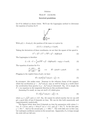
Let θ be defined as shown below. We’ll use the Lagrangian method to determine
the equation of motion for θ.
θ
l
m
y(t)
With y(t) = A cos(ωt), the position of the mass m is given by
(X, Y ) = ( sin θ, y + cos θ). (1)
Taking the derivatives of these coordinates, we see that the square of the speed is
V 2
= ˙X2
+ ˙Y 2
= 2 ˙θ2
+ ˙y2
− 2 ˙y ˙θ sin θ. (2)
The Lagrangian is therefore
L = K − U =
1
2
m( 2 ˙θ2
+ ˙y2
− 2 ˙y ˙θ sin θ) − mg(y + cos θ). (3)
The equation of motion for θ is
d
dt
∂L
∂ ˙θ
=
∂L
∂θ
=⇒ ¨θ − ¨y sin θ = g sin θ. (4)
Plugging in the explicit form of y(t), we have
¨θ + sin θ Aω2
cos(ωt) − g = 0. (5)
In retrospect, this makes sense. Someone in the reference frame of the support,
which has acceleration ¨y = −Aω2 cos(ωt), may as well be living in a world where
the acceleration from gravity is g − Aω2 cos(ωt) downward. Eq. (5) is simply the
F = ma equation in the tangential direction in this accelerated frame.
Assuming θ is small, we may set sin θ ≈ θ, which gives
¨θ + θ aω2
cos(ωt) − ω2
0 = 0, (6)
where ω0 ≡ g/ , and a ≡ A/ . Eq. (6) cannot be solved exactly, but we can still
get a good idea of how θ depends on time. We can do this both numerically and
(approximately) analytically.
The figures below show how θ depends on time for parameters with values =
1 m, A = 0.1 m, and g = 10 m/s2 (so a = 0.1, and ω2
0 = 10 s−2). In the first plot,
ω = 10 s−1. And in the second plot, ω = 100 s−1. The stick falls over in first case,
but undergoes oscillatory motion in the second case. Apparently, if ω is large enough
the stick will not fall over.
1
2. 0.2 0.4 0.6 0.8 1 1.2 1.4
t
0.1
0.05
0.05
0.1
theta
0.2 0.4 0.6 0.8 1 1.2 1.4
t
0.25
0.5
0.75
1
1.25
1.5
1.75
theta
Let’s now explain this phenomenon analytically. At first glance, it’s rather sur-
prising that the stick stays up. It seems like the average (over a few periods of the ω
oscillations) of the tangential acceleration in eq. (6), namely −θ(aω2 cos(ωt) − ω2
0),
equals the positive quantity θω2
0, because the cos(ωt) term averages to zero (or so
it appears). So you might think that there is a net force making θ increase, causing
the stick fall over.
The fallacy in this reasoning is that the average of the −aω2θ cos(ωt) term is not
zero, because θ undergoes tiny oscillations with frequency ω, as seen below. Both
of these plots have a = 0.005, ω2
0 = 10 s−2, and ω = 1000 s−1 (we’ll work with small
a and large ω from now on; more on this below). The second plot is a zoomed-in
version of the first one near t = 0.
2 4 6 8
t
0.1
0.05
0.05
0.1
theta
0.02 0.04 0.06 0.08 0.1
t
0.098
0.0985
0.099
0.0995
theta
The important point here is that the tiny oscillations in θ shown in the second
plot are correlated with cos(ωt). It turns out that the θ value at the t where
cos(ωt) = 1 is larger than the θ value at the t where cos(ωt) = −1. So there is a
net negative contribution to the −aω2θ cos(ωt) part of the acceleration. And it may
indeed be large enough to keep the pendulum up, as we will now show.
To get a handle on the −aω2θ cos(ωt) term, let’s work in the approximation
where ω is large and a ≡ A/ is small. More precisely, we will assume a 1 and
aω2 ω2
0, for reasons we will explain below. Look at one of the little oscillations
in the second of the above plots. These oscillations have frequency ω, because they
are due simply to the support moving up and down. When the support moves
up, θ increases; and when the support moves down, θ decreases. Since the average
position of the pendulum doesn’t change much over one of these small periods, we
can look for an approximate solution to eq. (6) of the form
θ(t) ≈ C + b cos(ωt), (7)
2
3. where b C. C will change over time, but on the scale of 1/ω it is essentially
constant, if a ≡ A/ is small enough.
Plugging this guess for θ into eq. (6), and using a 1 and aω2 ω2
0, we find
that −bω2 cos(ωt) + Caω2 cos(ωt) = 0, to leading order.1 So we must have b = aC.
Our approximate solution for θ is therefore
θ ≈ C 1 + a cos(ωt) . (8)
Let’s now determine how C gradually changes with time. From eq. (6), the
average acceleration of θ, over a period T = 2π/ω, is
¨θ = −θ aω2 cos(ωt) − ω2
0
≈ −C 1 + a cos(ωt) aω2 cos(ωt) − ω2
0
= −C a2
ω2
cos2(ωt) − ω2
0
= −C
a2ω2
2
− ω2
0
≡ −CΩ2
, (9)
where
Ω =
a2ω2
2
−
g
. (10)
But if we take two derivatives of eq. (7), we see that ¨θ simply equals ¨C. Equating
this value of ¨θ with the one in eq. (9) gives
¨C(t) + Ω2
C(t) ≈ 0. (11)
This equation describes nice simple-harmonic motion. Therefore, C oscillates sinu-
soidally with the frequency Ω given in eq. (10). This is the overall back and forth
motion seen in the first of the above plots. Note that we must have aω >
√
2ω0 if
this frequency is to be real so that the pendulum stays up. Since we have assumed
a 1, we see that a2ω2 > 2ω2
0 implies aω2 ω2
0, which is consistent with our
initial assumption above.
If aω ω0, then eq. (10) gives Ω ≈ aω/
√
2. Such is the case if we change
the setup and simply have the pendulum lie flat on a horizontal table where the
acceleration from gravity is zero. In this limit where g is irrelevant, dimensional
analysis implies that the frequency of the C oscillations must be a multiple of ω,
because ω is the only quantity in the problem with units of frequency. It just so
happens that the multiple is a/
√
2.
1
The reasons for the a 1 and aω2
ω2
0 qualifications are the following. If aω2
ω2
0, then the
aω2
cos(ωt) term dominates the ω2
0 term in eq. (6). The one exception to this is when cos(ωt) ≈ 0,
but this occurs for a negligibly small amount of time if aω2
ω2
0. If a 1, then we can legally
ignore the ¨C term when eq. (7) is substituted into eq. (6). We will find below, in eq. (9), that our
assumptions lead to ¨C being roughly proportional to a2
ω2
. Since the other terms in eq. (6) are
proportional to aω2
, we need a 1 in order for the ¨C term to be negligible. In short, a 1 is the
condition under which C varies slowly on the time scale of 1/ω.
3