Compression: Video Compression (MPEG and others)

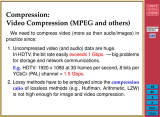
1. 446
Back
Close
Compression:
Video Compression (MPEG and others)
We need to compress video (more so than audio/images) in
practice since:
1. Uncompressed video (and audio) data are huge.
In HDTV, the bit rate easily exceeds 1 Gbps. — big problems
for storage and network communications.
E.g. HDTV: 1920 x 1080 at 30 frames per second, 8 bits per
YCbCr (PAL) channel = 1.5 Gbps.
2. Lossy methods have to be employed since the compression
ratio of lossless methods (e.g., Huffman, Arithmetic, LZW)
is not high enough for image and video compression.

2. 447
Back
Close
Not the complete picture studied here
Much more to MPEG — Plenty of other tricks employed.
We only concentrate on some basic principles of video
compression:
• Earlier H.261 and MPEG 1 and 2 standards.
with a brief introduction of ideas used in new standards such
as H.264 (MPEG-4 Advanced Video Coding).
Compression Standards Committees
Image, Video and Audio Compression standards have been
specified and released by two main groups since 1985:
ISO - International Standards Organisation: JPEG, MPEG.
ITU - International Telecommunications Union: H.261 — 264.

3. 448
Back
Close
Compression Standards
Whilst in many cases one of the groups have specified separate
standards there is some crossover between the groups.
For example:
• JPEG issued by ISO in 1989 (but adopted by ITU as ITU T.81)
• MPEG 1 released by ISO in 1991,
• H.261 released by ITU in 1993 (based on CCITT 1990 draft).
CCITT stands for Comit´e Consultatif International T´el´ephonique et
T´el´egraphique (International Telegraph and Telephone Consultative Committee)
whose parent organisation is ITU.
• H.262 is alternatively better known as MPEG-2 released in 1994.
• H.263 released in 1996 extended as H.263+, H.263++.
• MPEG 4 release in 1998.
• H.264 releases in 2002 to lower the bit rates with comparable quality video and
support wide range of bit rates, and is now part of MPEG 4 (Part 10, or AVC –
Advanced Video Coding).

4. 449
Back
Close
How to compress video?
Basic Idea of Video Compression:
Motion Estimation/Compensation
• Spatial Redundancy Removal – Intraframe coding (JPEG)
NOT ENOUGH BY ITSELF?
• Temporal — Greater compression by noting the temporal
coherence/incoherence over frames. Essentially we note the
difference between frames.
• Spatial and Temporal Redundancy Removal – Intraframe and
Interframe coding (H.261, MPEG)

5. 450
Back
Close
Simple Motion Estimation/Compensation
Example
Things are much more complex in practice of course.
Which Format to represent the compressed data?
• Simply based on Differential Pulse Code Modulation (DPCM).

6. 451
Back
Close
Simple Motion Example (Cont.)
Consider a simple image (block) of a moving circle.
Lets just consider the difference between 2 frames.
It is simple to encode/decode:

7. 452
Back
Close
Now lets Estimate Motion of blocks
We will examine methods of estimating motion vectors in
due course.

8. 453
Back
Close
Decoding Motion of blocks
Why is this a better method than just frame differencing?

9. 454
Back
Close
How is Block Motion used in Compression?
Block Matching:
• MPEG-1/H.261 is done by using block matching techniques,
For a certain area of pixels in a picture:
• find a good estimate of this area in a previous (or in a future)
frame, within a specified search area.
Motion compensation:
• Uses the motion vectors to compensate the picture.
• Parts of a previous (or future) picture can be reused in a
subsequent picture.
• Individual parts spatially compressed — JPEG type
compression

10. 455
Back
Close
Any Overheads?
• Motion estimation/compensation techniques reduces the
video bitrate significantly
but
• Introduce extras computational complexity and delay (?),
– Need to buffer reference pictures - backward and forward
referencing.
– Reconstruct from motion parameters
Lets see how such ideas are used in practice.

11. 456
Back
Close
H.261 Compression
The basic approach to H. 261 Compression is summarised as
follows:
H. 261 Compression has been specifically designed for video
telecommunication applications:
• Developed by CCITT in 1988-1990
• Meant for videoconferencing, videotelephone applications
over ISDN telephone lines.
• Baseline ISDN is 64 kbits/sec, and integral multiples (px64)

12. 457
Back
Close
Overview of H.261
• Frame types are CCIR 601 CIF (Common Intermediate Format)
(352x288) and QCIF (176x144) images with 4:2:0 subsampling.
• Two frame types:
Intraframes (I-frames) and Interframes (P-frames)
• I-frames use basically JPEG — but YUV (YCrCb) and larger
DCT windows, different quantisation
• I-frames provide us with a refresh accessing point — Key
Frames
• P-frames use pseudo-differences from previous
frame (predicted), so frames depend on each other.

13. 458
Back
Close
H.261 Group of Pictures
• We typically have a group of pictures — one I-frame followed by
several P-frames — a group of pictures
• Number of P-frames followed by each I-frame determines the size
of GOP – can be fixed or dynamic. Why this can’t be too large?

14. 459
Back
Close
Intra Frame Coding
• Various lossless and lossy compression techniques use —
like JPEG.
• Compression contained only within the current frame
• Simpler coding – Not enough by itself for high compression.
• Cant rely on intra frame coding alone not enough compression:
– Motion JPEG (MJPEG) standard does exist — not
commonly used.
– So introduce idea of inter frame difference coding
• However, cant rely on inter frame differences across a large
number of frames
– So when Errors get too large: Start a new I-Frame

15. 460
Back
Close
Intra Frame Coding (Cont.)
Intraframe coding is very similar to JPEG:
What are the differences between this and JPEG?

16. 461
Back
Close
Intra Frame Coding (Cont.)
A basic Intra Frame Coding Scheme is as follows:
• Macroblocks are typically 16x16 pixel areas on Y plane of
original image.
• A macroblock usually consists of 4 Y blocks, 1 Cr block, and
1 Cb block. (4:2:0 chroma subsampling)
– Eye most sensitive to luminance, less sensitive to chrominance.
∗ We operate on a more effective color space: YUV
(YCbCr) colour which we studied earlier.
– Typical to use 4:2:0 macroblocks: one quarter of the
chrominance information used.
• Quantization is by constant value for all DCT coefficients.
I.e., no quantization table as in JPEG.

17. 462
Back
Close
Inter-frame (P-frame) Coding
• Intra frame limited to spatial basis relative to 1 frame
• Considerable more compression if the inherent temporal basis
is exploited as well.
BASIC IDEA:
• Most consecutive frames within a sequence are very similar
to the frames both before (and after) the frame of interest.
• Aim to exploit this redundancy.
• Use a technique known as block-based motion compensated
prediction
• Need to use motion estimation
• Coding needs extensions for Inter but encoder can also
supports an Intra subset.

18. 463
Back
Close
Inter-frame (P-frame) Coding (Cont.)

19. 464
Back
Close
Inter-frame (P-frame) Coding (Cont.)
P-coding can be summarised as follows:

20. 465
Back
Close
Motion Vector Search
So we know how to encode a P-block.
How do we find the motion vector?

21. 466
Back
Close
Motion Estimation
• The temporal prediction technique used in MPEG video is
based on motion estimation.
The basic premise:
• Consecutive video frames will be similar except for changes
induced by objects moving within the frames.
• Trivial case of zero motion between frames — no other
differences except noise, etc.),
• Easy for the encoder to predict the current frame as a duplicate
of the prediction frame.
• When there is motion in the images, the situation is not as
simple.

22. 467
Back
Close
Example of a frame with 2 stick figures and
a tree
The problem for motion estimation to solve is :
• How to adequately represent the changes, or differences,
between these two video frames.

23. 468
Back
Close
Solution:
A comprehensive 2-dimensional spatial search is performed
for each luminance macroblock.
• Motion estimation is not applied directly to chrominance in
MPEG
• MPEG does not define how this search should be performed.
• A detail that the system designer can choose to implement
in one of many possible ways.
• Well known that a full, exhaustive search over a wide 2-D
area yields the best matching results in most cases, but at
extreme computational cost to the encoder.
• Motion estimation usually is the most computationally
expensive portion of the video encoding.

24. 469
Back
Close
Motion Estimation Example

25. 470
Back
Close
Motion Vectors, Matching Blocks
Previous figure shows an example of a particular macroblock
from Frame 2 of earlier example, relative to various macroblocks
of Frame 1:
• The top frame has a bad match with the macroblock to be
coded.
• The middle frame has a fair match, as there is some
commonality between the 2 macroblocks.
• The bottom frame has the best match, with only a slight error
between the 2 macroblocks.
• Because a relatively good match has been found, the encoder
assigns motion vectors to that macroblock,

26. 471
Back
Close
Final Motion Estimation Prediction

27. 472
Back
Close
Final Motion Estimation Prediction (Cont.)
Previous figure shows how a potential predicted Frame 2 can
be generated from Frame 1 by using motion estimation.
• The predicted frame is subtracted from the desired frame,
• Leaving a (hopefully) less complicated residual error frame
which can then be encoded much more efficiently than
before motion estimation.
• The more accurate the motion is estimated and matched,
the more likely it will be that the residual error will approach
zero — and the coding efficiency will be highest.

28. 473
Back
Close
Further coding efficiency
Differential Coding of Motion Vectors
• Motion vectors tend to be highly correlated between
macroblocks:
– The horizontal component is compared to the previously
valid horizontal motion vector and
∗ Only the difference is coded.
– Same difference is calculated for the vertical component
– Difference codes are then described with a variable length
code (e.g. Huffman) for maximum compression efficiency.

29. 474
Back
Close
RECAP: P-Frame Coding Summary

30. 475
Back
Close
What Happens if we can’t find acceptable
match?
P Blocks may not be what they appear to be?
If the encoder decides that no acceptable match exists then it
has the option of
• Coding that particular macroblock as an intra macroblock,
• Even though it may be in a P frame!
• In this manner, high quality video is maintained at a slight
cost to coding efficiency.

31. 476
Back
Close
Estimating the Motion Vectors
So How Do We Find The Motion?
Basic Ideas is to search for Macroblock (MB)
• Within a ±n x m pixel search window
• Work out Sum of Absolute Difference (SAD)
(or Mean Absolute Error (MAE) for each window but this is
computationally more expensive)
• Choose window where SAD/MAE is a minimum.

32. 477
Back
Close
Sum of Absolute Difference (SAD)
SAD is computed by:
For i = -n to +n
For j = -m to +m
SAD(i, j) = ΣN−1
k=0 ΣN−1
l=0
| C(x + k, y + l) − R(x + i + k, y + j + l) |
• N = size of Macroblock window typically (16 or 32 pixels),
• (x, y) the position of the original Macroblock, C, and
• R is the reference region to compute the SAD.
• C(x + k, y + l) – pixels in the macro block with upper left
corner (x, y) in the Target.
• R(X + i + k, y + j + l) – pixels in the macro block with upper
left corner (x + i, y + j) in the Reference.

33. 478
Back
Close
Mean Absolute Error (MAE)
• Cost function is:
MAE(i, j) = 1
N2 ΣN−1
k=0 ΣN−1
l=0
| C(x + k, y + l) − R(x + i + k, y + j + l) |
Search For Minimum
• Goal is to find a vector (u, v) such that SAD/MAE (u, v) is
minimum
– Full Search Method
– Two-Dimensional Logarithmic Search
– Hierarchical Search

34. 479
Back
Close
SAD Search Example
So for a ± 2x2 Search Area given by dashed lines and a 2x2
Macroblock window example, the SAD is given by bold dot dash
line (near top right corner):

35. 480
Back
Close
Full Search
• Search exhaustively the whole (2n + 1) × (2m + 1) window in
the Reference frame.
• A macroblock centred at each of the positions within the
window is compared to the macroblock in the target frame
pixel by pixel and their respective SAD (or MAE) is computed.
• The vector (i, j) that offers the least SAD (or MAE) is designated
as the motion vector (u, v) for the macroblock in the target
frame.
• Full search is very costly — assuming each pixel comparison
involves three operations (subtraction, absolute value, addition),
the cost for finding a motion vector for a single macroblock
is (2n + 1) · (2m + 1) · N2
· 3 = O(nmN2
).

36. 481
Back
Close
2D Logarithmic Search
• An approach takes several iterations akin to a binary search.
• Computationally cheaper, suboptimal but usually effective.
• Initially only nine locations in the search window are used as
seeds for a SAD(MAE)-based search (marked as ‘1’).
• After locating the one with the minimal SAD(MAE), the centre
of the new search region is moved to it and the step-size
(“offset”) is reduced to half.
• In the next iteration, the nine new locations are marked as
‘2’ and this process repeats.
• If L iterations are applied, for altogether 9L
positions, only 9L
positions are checked.

37. 482
Back
Close
2D Logarithmic Search (cont.)
2D Logarithmic Search for Motion Vectors

38. 483
Back
Close
Hierarchical Motion Estimation:
1. Form several low resolution version of the target and reference
pictures
2. Find the best match motion vector in the lowest resolution version.
3. Modify the motion vector level by level when going up

39. 484
Back
Close
Selecting Intra/Inter Frame coding
Based upon the motion estimation a decision is made on
whether INTRA or INTER coding is made.
To determine INTRA/INTER MODE we do the following
calculation:
MBmean =
ΣN−1
i=0,j=0|C(i,j)|
N2
A = ΣN−1
i=0,j=0 | C(i, j) − MBmean |
If A < (SAD − 2N) INTRA Mode is chosen.

40. 485
Back
Close
MPEG Compression
MPEG stands for:
• Motion Picture Expert Group — established circa 1990 to create
standard for delivery of audio and video
• MPEG-1 (1991).Target: VHS quality on a CD-ROM (320 x 240 +
CD audio @ 1.5 Mbits/sec)
• MPEG-2 (1994): Target Television Broadcast
• MPEG-3: HDTV but subsumed into an extension of MPEG-2
• MPEG 4 (1998): Very Low Bitrate Audio-Visual Coding, later
MPEG-4 Part 10(H.264) for wide range of bitrates and better
compression quality
• MPEG-7 (2001) “Multimedia Content Description Interface”
• MPEG-21 (2002) “Multimedia Framework”

41. 486
Back
Close
Three Parts to MPEG
• The MPEG standard had three parts:
1. Video: based on H.261 and JPEG
2. Audio: based on MUSICAM (Masking pattern adapted
Universal Subband Integrated Coding And Multiplexing)
technology
3. System: control interleaving of streams

42. 487
Back
Close
MPEG Video
MPEG compression is essentially an attempt to overcome
some shortcomings of H.261 and JPEG:
• Recall H.261 dependencies:

43. 488
Back
Close
The Need for a Bidirectional Search
• The Problem here is that many macroblocks need information
that is not in the reference frame.
• For example:
• Occlusion by objects affects differencing
• Difficult to track occluded objects etc.
• MPEG uses forward/backward interpolated prediction.

44. 489
Back
Close
MPEG B-Frames
• The MPEG solution is to add a third frame type which is a
bidirectional frame, or B-frame
• B-frames search for macroblock in past and future frames.
• Typical pattern is IBBPBBPBB IBBPBBPBB IBBPBBPBB
Actual pattern is up to encoder, and need not be regular.

45. 490
Back
Close
Example I, P, and B frames
Consider a group of pictures that lasts for 6 frames:
• Given: I,B,P,B,P,B,I,B,P,B,P,B,
• I frames are coded spatially only (as before in H.261).
• P frames are forward predicted based on previous I and P
frames (as before in H.261).
• B frames are coded based on a forward prediction from a
previous I or P frame, as well as a backward prediction
from a succeeding I or P frame.

46. 491
Back
Close
Example I, P, and B frames (Cont.)
• 1st B frame is predicted from the 1st I frame and 1st P frame.
• 2nd B frame is predicted from the 1st and 2nd P frames.
• 3rd B frame is predicted from the 2nd and 3rd P frames.
• 4th B frame is predicted from the 3rd P frame and the 1st I
frame of the next group of pictures.

47. 492
Back
Close
Backward Prediction Implications
Note: Backward prediction requires that the future frames
that are to be used for backward prediction be
• Encoded and Transmitted first, I.e. out of order.
This process is summarised:

48. 493
Back
Close
Backward Prediction Implications (Cont.)
Also NOTE:
• No defined limit to the number of consecutive B frames that
may be used in a group of pictures,
• Optimal number is application dependent.
• Most broadcast quality applications however, have tended
to use 2 consecutive B frames (I,B,B,P,B,B,P,) as the ideal
trade-off between compression efficiency and video quality.
• MPEG suggests some standard groupings.

49. 494
Back
Close
Advantage of the usage of B frames
• Coding efficiency.
• Most B frames use less bits.
• Quality can also be improved in the case of moving objects
that reveal hidden areas within a video sequence.
• Better Error propagation: B frames are not used to predict
future frames, errors generated will not be propagated further
within the sequence.
Disadvantage:
• Frame reconstruction memory buffers within the encoder and
decoder must be doubled in size to accommodate the 2
anchor frames.
• More delays in real-time applications.

50. 495
Back
Close
MPEG-2, MPEG-3, and MPEG-4
• MPEG-2 target applications
----------------------------------------------------------------
Level size Pixels/sec bit-rate Application
(Mbits)
----------------------------------------------------------------
Low 352 x 240 3 M 4 VHS tape equiv.
Main 720 x 480 10 M 15 studio TV
High 1440 1440 x 1152 47 M 60 consumer HDTV
High 1920 x 1080 63 M 80 film production
-----------------------------------------------------------------
• MPEG-2 differences from MPEG-1
1. Search on fields, not just frames.
2. 4:2:2 and 4:4:4 macroblocks
3. Frame sizes as large as 16383 x 16383
4. Scalable modes: Temporal, Progressive,...
5. Non-linear macroblock quantization factor
6. A bunch of minor fixes

51. 496
Back
Close
MPEG-2, MPEG-3, and MPEG-4 (Cont.)
• MPEG-3: Originally for HDTV (1920 x 1080), got folded into
MPEG-2
• MPEG-4: very low bit-rate communication (4.8 to 64 kb/sec).
Video processing
MATLAB MPEG Video Coding Code
MPEGVideo (DIRECTORY)
MPEGVideo.zip (All Files Zipped)

52. 497
Back
Close
MPEG-4 Video Compression
A newer standard than MPEG-2. Besides compression, great
attention is paid to issues about user interactivity.
We look at key ideas here.
• Object based coding: offers higher compression ratio, also
beneficial for digital video composition, manipulation, indexing
and retrieval.
• Synthetic object coding: supports 2D mesh object coding,
face object coding and animation, body object coding and
animation.
• MPEG-4 Part 10/H.264: new techniques for improved
compression efficiency.

53. 498
Back
Close
Object based coding (1)
Composition and manipulation of MPEG-4 videos.

54. 499
Back
Close
Object based coding (2)
Compared with MPEG-2, MPEG-4 is an entirely new standard
for
• Composing media objects to create desirable audiovisual
scenes.
• Multiplexing and synchronising the bitstreams for these
media data entities so that they can be transmitted with
guaranteed Quality of Service (QoS).
• Interacting with the audiovisual scene at the receiving end.
MPEG-4 provides a set of advanced coding modules and
algorithms for audio and video compressions.
We have discussed MPEG-4 Structured Audio and we will
focus on video here.

55. 500
Back
Close
Object based coding (3)
The hierarchical structure of MPEG-4 visual bitstreams is very
different from that of MPEG-2: it is very much
video object-oriented:

56. 501
Back
Close
Object based coding (4)
• Video-object Sequence (VS): delivers the complete MPEG4
visual scene; may contain 2D/3D natural or synthetic objects.
• Video Object (VO): a particular object in the scene, which
can be of arbitrary (non-rectangular) shape corresponding
to an object or background of the scene.
• Video Object Layer (VOL): facilitates a way to support
(multi-layered) scalable coding. A VO can have multiple VOLs
under scalable (multi-bitrate) coding, or have a single VOL
under non-scalable coding.
• Group of Video Object Planes (GOV): groups of video object
planes together (optional level).
• Video Object Plane (VOP): a snapshot of a VO at a particular
moment.

57. 502
Back
Close
VOP-based vs. Frame-based Coding
• MPEG-1 and MPEG-2 do not support the VOP concert; their
coding method is frame-based (also known as block-based).
• For block-based coding, it is possible that multiple potential
matches yield small prediction errors. Some may not coincide
with the real motion.
• For VOP-based coding, each VOP is of arbitrary shape and
ideally will obtain a unique motion vector consistent with the
actual object motion.
See the example in the next page:

58. 503
Back
Close
VOP-based vs. Frame-based Coding

59. 504
Back
Close
VOP-based Coding
• MPEG-4 VOP-based coding also employs
Motion Compensation technique:
– I-VOPs: Intra-frame coded VOPs.
– P-VOPs: Inter-frame coded VOPs if only forward prediction
is employed.
– B-VOPs: Inter-frame coded VOPs if bi-directional
predictions are employed.
• The new difficulty for VOPs: may have arbitrary shapes.
Shape information must be coded in addition to the texture
(luminance or chroma) of the VOP.

60. 505
Back
Close
VOP-based Motion Compensation (MC)
• MC-based VOP coding in MPEG-4 again involves three steps:
1. Motion Estimation
2. MC-based Prediction
3. Coding of the Prediction Error
• Only pixels within the VOP of the current (target) VOP are
considered for matching in MC. To facilitate MC, each VOP
is divided into macroblocks with 16 × 16 luminance and 8 × 8
chrominance images.

61. 506
Back
Close
VOP-based Motion Compensation (MC)
• Let C(x + k, y + l) be pixels of the MB in target in target VOP,
and R(x + i + k, y + j + l) be pixels of the MB in Reference
VOP.
• A Sum of Absolute Difference (SAD) for measuring the
difference between the two MBs can be defined as:
SAD(i, j) =
N−1
k=0
N−1
l=0
|C(x + k, y + l) − R(x + i + k, y + j + l)| · Map(x + k, y + l).
N — the size of the MB
Map(p, q) = 1 when C(p, q) is a pixel within the target VOP
otherwise Map(p, q) = 0.
• The vector (i, j) that yields the minimum SAD is adopted
as the motion vector (u, v).

62. 507
Back
Close
Coding of Texture and Shape
• Texture Coding (luminance and chrominance):
– I-VOP: the gray values of the pixels in each MB of the
VOP are directly coded using DCT followed by VLC
(Variable Length Coding), such as Huffman or Arithmetic
Coding.
– P-VOP/B-VOP: MC-based coding is employed — the
prediction error is coded similar to I-VOP.
– Boundary MBs need appropriate treatment. May also use
improved Shape Adaptive DCT.

63. 508
Back
Close
Coding of Texture and Shape (cont.)
• Shape Coding (shape of the VOPs)
– Binary shape information: in the form of a binary map.
A value ‘1’ (opaque) or ‘0’ (transparent) in the bitmap
indicates whether the pixel is inside or outside the VOP.
– Greyscale shape information: value refers to the
transparency of the shape ranging from 0 (completely
transparent) and 255 (opaque).
– Specific encoding algorithms are designed to code in both
cases.

64. 509
Back
Close
Synthetic Object Coding: 2D Mesh
• 2D Mesh Object: a tessellation (or partition) of a 2D planar
region using polygonal patches.
• Mesh based texture mapping can be used for 2D object
animation.

65. 510
Back
Close
Synthetic Object Coding: 3D Model
• MPEG-4 has defined special 3D models for face objects
and body objects because of the frequent appearances of
human faces and bodies in videos.
• Some of the potential applications: teleconferecing,
human-computer interfaces, games and e-commerce.
• MPEG-4 goes beyond wireframes so that the surfaces of the
face or body objects can be shaded or texture-mapped.

66. 511
Back
Close
Synthetic Object Coding: Face Object
Face Object Coding and Animation
• MPEG-4 adopted a generic default face model, developed
by VRML Consortium.
• Face Animation Parameters (FAPs) can be specified to
achieve desirable animation.
• Face Definition Parameters (FDPs): feature points better
describe individual faces.

67. 512
Back
Close
MPEG-4 Part 10/H.264
• Improved video coding techniques, identical standards: ISO
MPEG-4 Part 10 (Advanced Video Coding / AVC) and ITU-T
H.264.
• Preliminary studies using software based on this new standard
suggests that H.264 offers up to 30-50% better compression
than MPEG-2 and up to 30% over H.263+ and MPEG-4
advanced simple profile.
• H.264 is currently one of the leading candidates to carry
High Definition TV (HDTV) video content on many
applications, e.g. Blu-ray.
• Involves various technical improvements. We mainly look at
improved inter-frame encoding.

68. 513
Back
Close
MPEG-4 AVC: Flexible Block Partition
Macroblock in MPEG-2 uses 16×16 luminance values. MPEG-4
AVC uses a tree-structured motion segmentation down to 4 × 4
block sizes (16×16, 16×8, 8×16, 8×8, 8×4, 4×8, 4×4). This allows
much more accurate motion compensation of moving objects.

69. 514
Back
Close
MPEG-4 AVC: Up to Quarter-Pixel
Resolution Motion Compensation
Motion vectors can be up to half-pixel or quarter-pixel accuracy.
Pixels at quarter-pixel position are obtained by bilinear
interpolation.
• Improves the possibility of finding a block in the reference
frame that better matches the target block.

70. 515
Back
Close
MPEG-4 AVC: Multiple References
• Multiple references to motion estimation. Allows finding the
best reference in 2 possible buffers (past pictures and future
pictures) each contains up to 16 frames.
• Block prediction is done by a weighted sum of blocks from
the reference picture. It allows enhanced picture quality in
scenes where there are changes of plane, zoom, or when
new objects are revealed.

71. 516
Back
Close
Further Reading
• Overview of the MPEG-4 Standard
• The H.264/MPEG4 AVC Standard and its Applications