Inventory Reduction Benefits of Risk Pooling as a function of pairwise correlation estimates

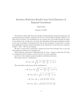
1. Inventory Reduction Benefits from Good Estimates of
Regional Correlations
Ashwin Rao
January 10, 2017
The literature often talks about the benefits of risk-pooling by reducing warehouses and
demonstrating the inventory reduction for the case of uncorrelated demand. However, we
know that in practice, the correlations are not exactly zero, but would typically be closer
to zero than to one. In this note, we derive the dependence of inventory-reduction benefits
on not just the number of warehouses but also on the correlation. In particular, we show
how significant inventory-reduction benefits can be obtained as we go from say correlation
of 20% → 10% → 0% for our business.
We have m stores and n warehouses. Assume the stores have demand N(µ, σ) per day
with pairwise-correlation of ρ among stores.
Each warehouse experiences withdrawal from m
n stores . Assume a lead time of L days
at a warehouse and we require a service level of α at each warehouse.
Let Φ(·) be the standard normal cumulative distribution function.
The safety stock at a warehouse is:
Φ−1
(α) ·
√
L ·
m
n
· σ2 + (
m
n
) · (
m
n
− 1) · σ2 · ρ
The total safety stock across all the warehouses is:
n · Φ−1
(α) ·
√
L ·
m
n
· σ2 + (
m
n
) · (
m
n
− 1) · σ2 · ρ
= Φ−1
(α) ·
√
L · σ · m · n · (1 + (
m
n
− 1) · ρ)
= Φ−1
(α) ·
√
L · σ · m · (n + (m − n) · ρ)
= Φ−1
(α) ·
√
L · σ · m · (m · ρ + n · (1 − ρ))
1

2. = Φ−1
(α) ·
√
L · σ · m · ρ +
n
m
· (1 − ρ)
Denoting the warehouses to stores ratio n
m as γ, the total safety stock across all the
warehouses can be written as:
= Φ−1
(α) ·
√
L · σ · m · ρ + γ · (1 − ρ)
Therefore, going from a higher correlation of ρ1 to a lower correlation of ρ2 gives us a
percentage reduction in the total safety stock across all the warehouses
= 1 −
ρ2 + γ · (1 − ρ2)
ρ1 + γ · (1 − ρ1)
As a practical example, assume stores m = 2000, warehouses n = 20(γ = 0.01), and ρ
reducing from 0.2 to 0.1.
Then, percentage reduction in total safety stock across all the warehouses is:
1 −
0.1 + 0.01 ∗ 0.9
0.2 + 0.01 ∗ 0.8
≈ 28%
And if ρ reduces from 0.2 to 0, the percentage reduction shoots up to:
1 −
0.0 + 0.01 ∗ 1.0
0.2 + 0.01 ∗ 0.8
≈ 78%
Further, if we assumed deeper risk-pooling with warehouses n = 10, we get even greater
inventory reduction benefits. The percentage reduction goes even higher to:
1 −
0.0 + 0.005 ∗ 1.0
0.2 + 0.005 ∗ 0.8
≈ 84%
This non-linear dependence on ρ can be taken advantage of by obtaining good estimates
of the correlation. The lower the upper-bound on the correlation, the more-accelerated the
inventory reduction benefits.
2