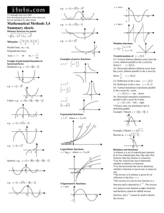
1. y = cos x
e.g. y = (x + 3)2 (x − 1)2
1
 Copyright itute.com 2006
0 π 2π
Free download & print from www.itute.com –3 0 1
Do not reproduce by other means
–1
Mathematical Methods 3,4 e.g. y = (x + 2 )3 (x − 1) y = tan x
Summary sheets
Distance between two points
–2 0 1 0 π 2π
= (x2 − x1 )2 + ( y2 − y1 )2
x +x y +y 
Mid-point =  1 2 , 1 2  e.g. y = (x + 2)4
 2 2  Modulus functions
Parallel lines, m1 = m2  x, x ≥ 0
y= x =
Perpendicular lines, − x , x < 0
1 –2 0
m1m2 = −1 or m2 = − Transformations of y = f (x )
m1
Examples of power functions: (1) Vertical dilation (dilation away from the
Graphs of polynomial functions in x-axis, dilation parallel to the y-axis) by
 1
factorised form: y = x −1  y =  factor k. y = kf (x )
Quadratics e.g. y = (x + 1)(x − 3)  x
(2) Horizontal dilation (dilation away from
0 the y-axis, dilation parallel to the x-axis) by
1
factor . y = f (nx )
n
–1 0 3
(3) Reflection in the x-axis. y = − f (x )
y = x −2 (4) Reflection in the y-axis. y = f (− x )
e.g. y = (x − 3)2
 1  (5) Vertical translation (translation parallel
y = 2
  to the y-axis) by c units.
 x 
y = f (x ) ± c , + up, – down.
0
0 3 1
(6) Horizontal translation (translation
Cubics e.g. y = 3(x + 1)(x − 1)(x − 2 ) y= x2
parallel to the x-axis) by b units.
y = f (x ± b ) , + left, – right.
(y = x ) *Always carry out translations last in
0 sketching graphs.
Example 1 Sketch y = − 2(x − 1) + 2
Exponential functions:
-1 0 1 2 2
y = a x where a = 2, e,10
0 1 2
e.g. y = (x + 1)2 (x − 1)
10x ex 2x
–1 0 1 Example 2 Sketch y = 2 1 − x .
Rewrite as y = 2 − (x − 1) .
1 2
asymptotic 0
e.g. y = (x + 1) 3
0 1
Logarithmic functions: Relations and functions:
–1 0 y = log a x where a = 2, e,10 A relation is a set of ordered pairs (points).
If no two ordered pairs have the same first
2x element, then the relation is a function.
Quartics e.g. y = (x + 3)(x + 1)(x − 1)(x − 2 ) ex *Use the vertical line test to determine
whether a relation is a function.
10x *Use the horizontal line test to determine
–3 –1 0 1 2 0 1 whether a function is one-to-one or many-to-
asymptotic one.
*The inverse of a relation is given by its
reflection in the line y = x .
*The inverse of a one-to-one function is a
e.g. y = (x + 3)2 (x − 1)(x − 2 ) Trigonometric functions: function and is denoted by f −1 . The inverse
y = sin x
of a many-to-one function is not a function
1
and therefore cannot be called inverse
–3 0 1 2 0 π 2π function, and f −1 cannot be used to denote
the inverse.
–1

2. Factorisation of polynomials: Quadratic formula: Index laws:
( )
(1) Check for common factors first. 2
Solutions of ax + bx + c = 0 are am n
(2) Difference of two squares, a ma n = a m+ n , = am−n , am = a mn
an
( ) − 3 = (x − 3)(x + 3)
2
2 − b ± b − 4ac
e.g. x 4 − 9 = x 2 2 2 2 x= . 1 1
(ab )n = a nbn , = a−n , am =
( 3 )(x + 3 )(x + 3)
2a
= x− 2 n −m
Graphs of transformed trig. functions a a
(3) Trinomials, by trial and error,  π 1 1
e.g. y = −2 cos 3 x −  + 1 , rewrite a 0 = 1, a 2 =na
e.g. 2 x 2 − x − 1 = (2 x + 1)(x − 1)  2 = a,a n
(4) Difference of two cubes, e.g.  π
( )
Logarithm laws:
equation as y = −2 cos 3 x −  + 1 .
x3 − y 3 = (x − y ) x 2 + xy + y 2  6 a
log a + log b = log ab, log a − log b = log
3 b
(5) Sum of two cubes, e.g. 8 + a = The graph is obtained by reflecting it in the
(
23 + a3 = (2 + a ) 4 − 2a + a 2 ) x-axis, dilating it vertically so that its
amplitude becomes 2, dilating it horizontally log ab = b log a, log
1
b
= − log b, log a a = 1
(6) Grouping two and two, 2π
e.g. x3 + 3x 2 + 3 x + 1 = x3 + 1 + 3 x 2 + 3 x( ) ( ) so that its period becomes
3
, translating log1 = 0, log 0 = undef , log(neg ) = undef
(
= (x + 1) x − x + 1 + 3 x(x + 1)
2
) upwards by 1 and right by
π
.
Change of base:
= (x + 1)(x ) 6 log b x
2
− x + 1 + 3x log a x = ,
log b a
= (x + 1)(x+ 2 x + 1 = (x + 1)3
2
) 3 log e 7
(7) Grouping three and one, e.g. log 2 7 = = 2.8 .
log e 2
e.g. x 2 − 2 x − y 2 + 1 π 5π
0 Exponential equations:
( )
= x 2 − 2 x + 1 − y 2 = (x − 1)2 − y 2 –1
6 6
e.g. 2e3 x = 5, e3 x = 2.5 , 3x = loge 2.5 ,
= (x − 1 − y )(x − 1 + y ) 1
(8) Completing the square, e.g. x= loge 2.5
3
1 1
2 2 Solving trig. equations
x2 + x −1 = x2 + x +   −   −1 e.g. 2e 2 x − 3e x − 2 = 0 ,
2  2 3
2  
2
e.g. Solve sin 2 x =
2
, 0 ≤ x ≤ 2π .
( ) − 3(e )− 2 = 0 ,
2 ex
2 x

=  x2


+x+
1
−
4

5
4

=x +


1

2

−

 2
5 


∴ 0 ≤ 2 x ≤ 4π ,
π 2π π 2π
(2e + 1)(e − 2) = 0 , since 2e
x x x
+1 ≠ 0 ,
 
2x = , , + 2π , + 2π x x
∴ e − 2 = 0 , e = 2 , x = loge 2 .
 3 3 3 3
1 5  
 x + 1 + 5 
= x +
 −  π π 7π 4π
 2 2  2 2 
 ∴x = , , , . Equations involving log:
   6 3 6 3 e.g. loge (1 − 2 x ) + 1 = 0 , loge (1 − 2 x ) = −1 ,
(9) Factor theorem, x x
e.g. sin = 3 cos , 0 ≤ x ≤ 2π . 1 1
e.g. P(x ) = x3 − 3x 2 + 3 x − 1 2 2 1 − 2 x = e −1 , 2 x = 1 − e −1 , x = 1 −  .
2 e
P(− 1) = (− 1)3 − 3(− 1)2 + 3(− 1) − 1 ≠ 0 sin
x
e.g. log10 (x − 1) = 1 − log10 (2 x − 1)
x 2 = 3 , tan x = 3 ,
P(1) = 13 − 3(1)2 + 3(1) − 1 = 0 0 ≤ ≤π,
x log10 (x − 1) + log10 (2 x − 1) = 1
2 2
∴ (x − 1) is a factor. cos
2 log10 (x − 1)(2 x − 1) = 1 , (x − 1)(2 x − 1) = 10 ,
Long division: x π 2π
∴ = , ∴x = . 2 x 2 − 3x − 9 = 0 , (2 x + 3)(x − 3) = 0 ,
x2 − 2x + 1 2 3 3 3
x − 1)x3 − 3 x 2 + 3 x − 1 x = − , 3 . 3 is the only solution because
2
(
− x3 − x 2 ) Exact values for trig. functions:
x=−
3
makes the log equation undefined.
− 2 x 2 + 3x xo x sin x cos x tan x 2
(
− − 2x2 + 2 x ) 0
30
0
π/6
0
1/2
1
√3/2
0
1/√3 Equation of inverse:
x −1 Interchange x and y in the equation to obtain
45 π/4 1/√2 1/√2 1
− (x − 1) 60 π/3 √3/2 1/2 √3
the equation of the inverse. If possible
express y in terms of x.
0 90 π/2 1 0 undef
(
∴ P(x ) = (x − 1) x 2 − 2 x + 1 = (x − 1)3 ) 120 2π/3 √3/2 –1/2 –√3
e.g. y = 2(x − 1)2 + 1 , x = 2( y − 1)2 + 1 ,
x −1
135 3π/4 1/√2 –1/√2 –1 2( y − 1)2 = x − 1 , ( y − 1)2 = ,
Remainder theorem: 150 5π/6 1/2 –√3/2 –1/√3 2
e.g. when P (x ) = x3 − 3 x 2 + 3 x − 1 is 180 π 0 –1 0 x −1
210 7π/6 –1/2 –√3/2 1/√3 y=± +1 .
divided by x + 2 , the remainder is 2
225 5π/4 –1/√2 –1/√2 1
P (− 2) = (− 2)3 − 3(− 2)2 + 3(− 2) − 1 = −11 240 4π/3 –√3/2 –1/2 √3 e.g. y = −
2
+4, x = −
2
+4 ,
When it is divided by 2 x − 3 , the remainder x −1 y −1
270 3π/2 –1 0 undef
3 1 300 5π/3 –√3/2 1/2 –√3 2 2
is P  = . x−4= − , y −1 = − ,
2 8 315 7π/4 –1/√2 1/√2 –1 y −1 x−4
330 11π/6 –1/2 √3/2 –1/√3 2
y=− +1 .
360 2π 0 1 0 x−4

3. e.g. y = −2e x −1 + 1 , x = −2e y −1 + 1 , Differentiation rules: The approx. change in a function is
The product rule: For the multiplication of = f (a + h ) − f (a ) = hf ′(a ) ,
1− x
2e y −1 = 1 − x , e y −1 = , two functions, y = u (x )v(x ) , e.g. e.g. find the approx. change in cos x when x
2
y = x 2 sin 2 x , let u = x 2 , v = sin 2 x , π
1− x  1− x  changes from to 1.6. Let f (x ) = cos x ,
y − 1 = loge   , y = log e   +1. dy du dv 2
 2   2  =v +u π
dx dx dx then f ′(x ) = − sin x . Let a = , then
e.g. y = − loge (1 − 2 x ) − 1 , ( )
= (sin 2 x )(2 x ) + x 2 (2 cos 2 x )
π
2
π
x = − loge (1 − 2 y ) − 1 , = 2 x(sin 2 x + x cos 2 x ) f ′(a ) = − sin = −1 and h = 1.6 − = 0.03
2 2
The quotient rule: For the division of
loge (1 − 2 y ) = −(x + 1) , 1 − 2 y = e − ( x +1) u (x ) log e x Change in cos x = hf ′(a ) = 0.03×− 1 = −0.03
functions, y = , e.g. y = ,
1
2
(
2 y = 1 − e − ( x +1) , y = 1 − e − ( x +1) .) v(x ) x Rate of change:
dy
dx
is the rate of change of
du dv
The binomial theorem: v −u dx
dy dx dx
= y with respect to x. v = , velocity is the
e.g. Expand (2 x − 1)4 dx v2 dt
= 4C0 (2 x )4 (− 1)0 + 4C1 (2 x )3 (− 1)1 rate of change of position x with respect to
(x ) 1  − (loge x )(1)
  dv
+ 4C2 (2 x )2 (− 1)2 + 4C3 (2 x )1 (− 1)3 x 1 − log e x time t. a = , acceleration a is the rate of
=   2 = . dt
x x2
+ 4C4 (2 x )0 (− 1)4 = ...... The chain rule: For composite functions,
change of velocity v with respect to t.
e.g. Find the coefficient of x2 in the
y = f (u ( x) ) , e.g. y = e cos x . Average rate of change: Given y = f (x ) ,
expansion of (2 x − 3)5 .
dy dy du when x = a , y = f (a ) , when x = b ,
Let u = cos x , y = eu , = ×
The required term is 5C3 (2 x )2 (− 3)3 dx du dx y = f (b ) , the average rate of change of y
( )
= 10 4 x 2 (− 27 ) = −1080 x 2 . ( )( sin x) = −e
= eu − cos x
sin x . with respect to x =
∆y
=
f (b ) − f (a )
.
∴ the coefficient of x2 is –1080. dy ∆x b−a
Finding stationary points: Let = 0 and
dx
Differentiation rules: solve for x and then y, the coordinates of the Deducing the graph of gradient function
dy from the graph of a function
y = f (x ) = f ' (x ) stationary point.
f(x)
dx Nature of stationary point at x = a :
•
ax n anx n −1 Local Local Inflection
•
max. min. point
a(x + c )n an(x + c )n −1 x<a dy dy dy
0 x
>0 <0 > 0 , (< 0)
a(bx + c )n abn(bx + c )n −1 dx dx dx
x=a dy dy dy
a sin x a cos x =0 =0 =0 o
dx dx dx
a sin (x + c ) a cos(x + c ) x>a dy dy dy f’(x)
a sin (bx + c ) ab cos(bx + c ) <0 >0 > 0 , (< 0)
dx dx dx o o
a cos x −a sin x Equation of tangent and normal at x = a :
•
a cos(x + c ) − a sin (x + c ) 1) Find the y coordinate if it is not given. 0 o x
dy
a cos(bx + c ) − ab sin (bx + c ) 2) Gradient of tangent mT = at x = a . •
dx
a tan x a sec 2 x 3) Use y − y1 = mT (x − x1 ) to find equation Deducing the graph of function from the
a tan (x + c ) a sec (x + c )
2 of tangent. graph of anti-derivative function
a tan (bx + c )
1
ab sec 2 (bx + c ) 4) Find gradient of normal mN = − . ∫ f(x)dx+ c
mT
x x
ae ae 5) Use y − y1 = m N (x − x1 ) to find equation •
x+c
ae ae x + c of the normal. •
Linear approximation: 0 x
ae bx + c abe bx + c To find the approx. value of a function, use
a log e x a f (a + h ) ≈ f (a ) + hf ′(a ) , e.g. find the
x approx. value of 25.1 . Let f (x ) = x ,
o
a log e bx a 1
x then f ′(x ) = . Let a = 25 and h = 0.1 , f(x)
2 x o o
a log e (x + c ) a
then f (a + h ) = 25.1 , f (a ) = 25 = 5 ,
x+c 0 o • x
1
a log e b(x + c ) a f ′(a ) = = 0.1 .
2 25 •
x+c
∴ 25.1 ≈ 5 + 0.1 × 0.1 = 5.01
a log e (bx + c ) ab
bx + c

4. Anti-differentiation (indefinite integrals): Estimate area by left (or right) rectangles Graphics calculator :
Pr ( X = a ) = binompdf (n, p, a )
f (x )
∫ f (x)dx Left Right Pr ( X ≤ a ) = binomcdf (n, p, a )
ax n for n ≠ −1 a n +1
x a b a b Pr ( X < a ) = binomcdf (n, p, a − 1)
n +1 Area between two curves: Pr ( X ≥ a ) = 1 − binomcdf (n, p, a − 1)
a (x + c )n , n ≠ −1 a
(x + c )n +1 y = g (x ) Pr ( X > a ) = 1 − binomcdf (n, p, a )
n +1 y = f (x ) Pr (a ≤ X ≤ b ) = binomcdf (n, p, b )
a (bx + c )n , n ≠ −1 a
(bx + c )n +1 a 0 b −binomcdf (n, p, a − 1)
(n + 1)b Probability density functions f (x ) for
a a log e x , x > 0 x ∈ [a, b] . y y = f (x )
x a log e (− x ) , x < 0 Firstly find the x-coordinates of the
a a log e (x + c ) intersecting points, a, b, then evaluate
b a c b x
x+c
a a
log e (bx + c )
A=
∫ [ f (x) − g (x)]dx . Always the function
a
For f (x ) to be a probability density
above minus the function below. function, f (x ) > 0 and
bx + c b b
For three intersecting points:
ae x ae x Pr (a < X < b ) =
∫ f (x)dx = 1.
a
ae x + c ae x + c y = f (x ) c b
ae bx + c a bx + c
e
y = g (x ) Pr ( X < c ) =
∫ f (x)dx , Pr(X > c) = ∫ f (x)dx
a c
b a b 0 c Normal distributions are continuous prob.
a sin x − a cos x distributions. The graph of a normal dist. has
b c
a sin (x + c ) − a cos(x + c )
∫ [ f (x) − g (x)]dx ∫ [g (x) − f (x )]dx
a bell shape and the area under the graph
A= +
represents probability. Total area = 1.
a sin (bx + c )
a b
a
− cos(bx + c )
b
Discrete probability distributions: ( )
N 1 µ1 , σ 2 , N 2 µ 2 , σ 2 . ( )
In general, in the form of a table,
a cos x a sin x x x1 x2 x3 ...... 1 2 µ1 < µ 2
a cos(x + c ) a sin (x + c )
Pr ( X = x ) p1 p2 p3 ......
a cos(bx + c ) a 0 µ1 µ2 X
sin (bx + c ) p1 , p2 , p3 ,... have values from 0 to 1 and
b
p1 + p2 + p3 + ... = 1 . ( 2
)
N1 µ , σ 1 , N 2 µ , σ 2 ( 2
).
Definite integrals: µ = E ( X ) = x1 p1 + x2 p2 + x3 p3 + ... 1 σ1 < σ 2
π π
Var ( X ) = x1 p1 + x2 p2 + x3 p3 + ... − µ 2
2 2 2 2
 π   π  2
e.g.
∫
0
2 cos x − dx = sin  x − 
 3   3  0 σ = sd ( X ) = Var ( X )
0 X
π π   π If random variable Y = aX + b ,
= sin  −  − sin  0 −  The standard normal distribution:
2 3  3 E (Y ) = aE ( X ) + b , Var (Y ) = a 2 × Var ( X ) has µ = 0 and σ = 1 . N (0,1)
and sd (Y ) = a × sd ( X ) .
π  π  1+ 3
= sin − sin  −  = . 95% probability interval : (µ − 2δ , µ + 2δ ) µ σ 2
6  3 2
Pr ( A ∩ B )
Properties of definite integrals: Conditional prob: Pr A B = ( ) Pr (B )
.
b b
1)
∫ kf (x)dx = k ∫ f (x)dx
a a
Binomial distributions are examples of
discrete prob. distributions. Sampling with
0 Z
b b b Graphics calculator: Finding probability,
2) [ f (x ) ± g (x )]dx = f (x )dx ± g (x )dx
∫ ∫ ∫
replacement has a binomial distribution.
a a a Number of trials = n. In a single trial, prob. Pr ( X < a ) = normalcdf (− E 99, a, µ , σ )
b c b of success = p, prob. of failure = q = 1- p. Pr ( X > a ) = normalcdf (a, E 99, µ , σ )
∫ a ∫ ∫
3) f (x )dx = f (x )dx + f (x )dx ,
a c
The random variable X is the number of
successes in the n trials. The binomial dist.
Pr (a < X < b ) = normalcdf (a, b, µ , σ )
b a Finding quantile, e.g. given Pr ( X < x ) = 0.7
is Pr ( X = x )= n C x p x q n− x , x = 0,1,2,... with
∫ ∫
where a < c < b . 4) f (x )dx = − f (x )dx
a b x = invNorn(0.7, µ , σ ) .
b a a µ = np and σ = npq = np(1 − p ) . Given Pr ( X > x ) = 0.7 , then
∫ a ∫ b∫
4) f (x )dx = − f (x )dx , 5) f (x )dx = 0.
a
** Effects of increasing n on the graph of a Pr ( X < x ) = 1 − 0.7 = 0.3 and
Area ‘under’ curve: binomial distribution. (1) more points x = invNorm(0.3, µ , σ ) .
(2) lower probability for each x value
(3) becoming symmetrical , bell shape. X −µ
b To find µ and/or σ, use Z = to
y = f (x ) A=
∫ f (x)dx
a
** Effects of changing p on the graph of a
binomial distribution. (1) bell shape when
σ
convert X to Z first, e.g. find µ given σ = 2
a 0 b p = 0.5 (2) positively skewed if p < 0.5  4−µ
y = f (x ) and Pr ( X < 4) = 0.8 . Pr  Z <  = 0.8 ,
(3) negatively skewed if p > 0.5  2 
a c 0 b p = 0.5 p < 0.5 p > 0.5 4−µ
c b
∴ = invNorm(0.8) = 0.8416 ,
2
∫
A = − f (x )dx +
a ∫ f (x)dx
c ∴ µ = 2.3168 .