Theoretical Spectroscopy Lectures: real-time approach 1
•
2 gefällt mir•411 views

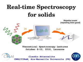
In this lecture, I will describe how to calculate optical response functions using real-time simulations. In particular, I will discuss td-hartree, td-dft and similar approximations.

Empfohlen
Empfohlen
Weitere ähnliche Inhalte
Was ist angesagt?
Was ist angesagt? (20)
Ähnlich wie Theoretical Spectroscopy Lectures: real-time approach 1
Ähnlich wie Theoretical Spectroscopy Lectures: real-time approach 1 (20)
Mehr von Claudio Attaccalite
Mehr von Claudio Attaccalite (20)
Kürzlich hochgeladen
Kürzlich hochgeladen (20)
Theoretical Spectroscopy Lectures: real-time approach 1
- 5. Why nonlinear optics? ..applications.. New green laser appeared in 2012 without nonlinear crystals
- 7. To see “invisible” excitations The Optical Resonances in Carbon Nanotubes Arise from Excitons Feng Wang, et al. Science 308, 838 (2005); ..research.. Right interpretation of the experiment “Selection rules for one-and two-photon absorption by excitons in carbon nanotubes,” E. B. Barros et al. PRB 73, 241406 (2006).
- 8. Probing symmetries Probing Symmetry Properties of Few-Layer MoS2 and h-BN by Optical Second-Harmonic Generation Nano Lett. 13, 3329 (2013) SHG can probe magnetic transition
- 13. What is realtime spectroscopy? Choose a perturbation E(t)=δ(t−t0) E0 E(t)=sin(ωt)E0 Timeevolution of an effective Schroedinger equation Ψ(t+Δt)=Ψ(t)−i Δ t H Ψ (t ) Ψ(t=0)=ΨGS
- 14. What is realtime spectroscopy? Choose a perturbation E(t)=δ(t−t0) E0 E(t)=sin(ωt)E0 Timeevolution of an effective Schroedinger equation Ψ(t+Δt)=Ψ(t)−i Δ t H Ψ (t ) Ψ(t=0)=ΨGS Analise the results
- 15. Real time spectroscopy in practice 1 3- / D(r ,t)=E(r ,t)+P(r ,t) Materials equations: Electric Displacement Electric Field Polarization ∇⋅E(r ,t)=4 πρtot (r ,t) ∇⋅D(r ,t)=4 πρext (r ,t) From Gauss's law: Δ P(r ,t)=∫χ(t−t ' ,r ,r ')E(t ' r ')dt ' dr '+∫dt 1 dt 2 χ 2 (...)E(t 1 ) E(t 2 )+O(E 3 ) In general:
- 16. Real time spectroscopy in practice 2 3- / For a small perturbation we consider only the first term, the linear response regime Δ P(r ,t)=∫χ(t−t ' ,r ,r ')E(t ' r ')dt ' dr '+O(E2 ) Δ P(ω)=χ(ω)E(ω)=(ϵ(ω)−1)E(ω) And finally: ϵ(ω)=1+ Δ P(ω) E(ω) ϵ(ω)= D(ω) E(ω)
- 17. Real time spectroscopy in practice 3 3- / 1) Choose an external perturbation E(t) 2) Evolve the Schroedinger equation 3) We calculate the P(t) from (t) 4) Fourier transform P(t) and E(t) and get i d Ψ(t ) dt =[H + E(t )]Ψ(t ) ϵ(ω)=1+ Δ P(ω) E(ω)
- 18. Motivations Better scaling for large system Polarization and Hamiltonian depend only from valence bands. No need of conduction bands!
- 19. Motivations Better scaling for large system Theory and implementation are much easier Polarization and Hamiltonian depend only on valence bands. No need of conduction bands!
- 20. One code to rule all spectroscopy responses χ(2) (ω;ω1, ω2) P(ω)=P0+χ (1) (ω)E1(ω)+χ (2) E1(ω1) E2(ω2)+χ (3) E1 E2 E3+O(E 4 ) SFG DFG SHG
- 21. One code to rule all spectroscopy responses χ(3) (ω; ω1, ω2, ω3) THG P(ω)=P0+χ(1) (ω)E1(ω)+χ(2) E1(ω1) E2(ω2)+χ(3) E1 E2 E3+O(E4 )
- 22. One code to rule all“ ” correlation effects Equation of motions are always the same In order to include correlation effects just change the Hamiltonian Notice that the present approach is limited to single-particle Hamiltonians. H=H1+H2+H3+...
- 24. The Hamiltonian I independent particles H KS(ρ0)=T+V ion+V h(ρ0)+V xc (ρ0) We start from the Kohn-Sham Hamiltonian If we keep fixed the density in the Hamiltoanian to the ground-state one we get the independent particle approximation In the Kohn-Sham basis this reads: H KS(ρ0)=ϵi KS δi, j
- 25. The Hamiltonian II timedependent Hartree (RPA) HTDH =T+Vion+V h(ρ)+V xc (ρ0) If we keep fixed the density in Vxc but not in Vh. We get the time-dependent Hartree or RPA (with local fields) Or equivalent: HTDH =H KS(ρ0)+Vh (ρ−ρ0) The density is written as: ρ(r ,t)=∑i=1 N v |Ψ(r ,t)| 2
- 26. The Hamiltonian III TDDFT HTDH =T+Vion+V h(ρ)+V xc (ρ) We let density fluctuate in both the Hartree and the Vxc tems We get the TD-DFT for solids The RungeGross theorem guarantees that this is an exact theory for isolated systems
- 27. Dephasing Gauge-independent decoherence models for solids in external fields M. S. Wismer and V. S. Yakovlev Phys. Rev. B 97, 144302 (2018) The previous Hamiltonian are Hermitian without any time-dependence (expect the external field) This means they do not introduce any dephasing! Dephasing as non-local operator in the Hamiltoanian Dephasing in post-(pre) processing ~P(t)=P(t)e−λ t See Octopus code or Y.Takimoto, Phd thesis (2008)
- 31. Non-linear optics in molecules Non-linear optics can calculated in the same way of TD-DFT as it is done in OCTOPUS or RT-TDDFT/SIESTA codes. Quasi-monocromatich-field p-nitroaniline Y.Takimoto, Phd thesis (2008)
- 32. Non-linear response in extended systems: a real-time approach Claudio Attaccalite https://arxiv.org/abs/1609.09639
- 33. External and total field
- 34. How to calculated the dielectric constant i ∂ ̂ρk (t) ∂t =[Hk +V eff , ̂ρk ] ̂ρk (t)=∑i f (ϵk ,i)∣ψi,k 〉〈 ψi,k∣ The Von Neumann equation (see Wiki http://en.wikipedia.org/wiki/Density_matrix) r t ,r' t' = ind r ,t ext r' ,t ' =−i〈[ r ,t r' t ']〉We want to calculate: We expand X in an independent particle basis set χ(⃗r t ,⃗r ' t ' )= ∑ i, j,l,m k χi, j,l,m, k ϕi, k (r)ϕj ,k ∗ (r)ϕl,k (r')ϕm ,k ∗ (r') χi, j,l,m, k= ∂ ̂ρi, j, k ∂Vl,m ,k Quantum Theory of the Dielectric Constant in Real Solids Adler Phys. Rev. 126, 413–420 (1962) What is Veff ?
- 35. Independent Particle Independent Particle Veff = Vext ∂ ∂Vl ,m,k eff i ∂ρi, j ,k ∂t = ∂ ∂Vl ,m, k eff [Hk+V eff , ̂ρk ]i, j, k Using: { Hi, j ,k = δi, j ϵi(k) ̂ρi, j, k = δi, j f (ϵi,k)+ ∂ ̂ρk ∂V eff ⋅V eff +.... And Fourier transform respect to t-t', we get: χi, j,l,m, k (ω)= f (ϵi,k)−f (ϵj ,k) ℏ ω−ϵj ,k+ϵi ,k+i η δj ,l δi,m i ∂ ̂ρk (t) ∂t =[Hk +V eff , ̂ρk ] χi, j,l,m, k= ∂ ̂ρi, j, k ∂Vl,m ,k
- 36. Optical Absorption: IP Non Interacting System δρNI=χ 0 δVtot χ 0 =∑ ij ϕi(r)ϕj * (r)ϕi * (r')ϕj(r ') ω−(ϵi−ϵj)+ i η Hartree, Hartree-Fock, dft. =ℑχ0=∑ ij ∣〈 j∣D∣i〉∣2 δ(ω−(ϵj −ϵi)) ϵ'' (ω)= 8 π 2 ω2 ∑ i, j ∣〈ϕi∣e⋅̂v∣ϕj 〉∣2 δ(ϵi−ϵj−ℏ ω) Absorption by independent Kohn-Sham particles Particles are interacting!
- 37. V ext= 0 V extV HV xc q ,= 0 q , 0 q,vf xc q ,q , TDDFT is an exact theory for neutral excitations! Time Dependent DFT V eff (r ,t)=V H (r ,t)+ V xc (r ,t)+ V ext (r ,t) Interacting System Non Interacting System Petersilka et al. Int. J. Quantum Chem. 80, 584 (1996) I= NI= I Vext 0= NI V eff ... by using ... = 0 1 V H V ext V xc V ext v f xc i ∂ ̂ρk (t) ∂t =[ HKS , ̂ρk ]=[ Hk 0 +V eff , ̂ρk ]