Cloud vertical distribution in extratropical cyclones poster

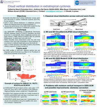
1. Cloud vertical distribution in extratropical cyclones
Catherine Naud (Columbia Univ.), Anthony Del Genio (NASA-GISS), Mike Bauer (Columbia Univ.) and
William Kovari (CCSR, Columbia Univ.). Contact: cnaud@giss.nasa.gov. J. Climate, in press.
Objectives 1. Classical cloud distribution across cold and warm fronts
Composite CloudSat cloud vertical distribution across warm
and cold fronts in oceanic midlatitude cyclones (30-70°N),
for two winters to:
1.Verify if cloud vertical distribution in midlatitude cyclones
follows the classical picture for frontal cloudiness (1).
2. Assess the performance of the GISS GCM model-E for the
representation of cloudiness in midlatitude cyclones
Technique Cold front Warm front
- Use NASA-MAP Climatology of Mid-latitude Storminess 2. NH and SH CloudSat-CALIPSO cloud distribution
(MCMS) database based on NCEP-2 reanalysis sea level Cold front Warm front
pressures to automatically detect midlatitude cyclones and
apply Hewson (1998) method to NCEP-2 850 mb potential
temperatures to detect warm and cold fronts
- Select CloudSat cloud observations when the orbit track
crossed a front and build composites of cloud frequency of
occurrence in a latitude-height grid across the fronts (2).
- Apply a similar technique onto GISS model-E (2ºx2.5ºx40L
version) outputs for 5 winter months (3).
Future work
Use ARM profiles of IWP/LWP, effective particle size and
integrated optical thickness (e.g. Mace et al. PI product) to
Slight difference with classical model: low-level clouds everywhere across cold and
study cloud properties across fronts
warm fronts, high level clouds ubiquitous across warm fronts and upright convection at
warm front. Solid line (left) = precipitation rates.
3. NH and SH GISS Model-E GCM cloud distribution
Cold front Warm front
General features of distribution close to observations but cloud fraction much smaller:
humidity not transported along vertical, resolution too coarse => GCM storms too
shallow and frontal motion not resolved. Solid line (left) = precipitation rates.
Example of cyclone for 2008-01-14, 18UTC,
40.83oN and 65.98oW 4. Problems with moisture vertical transport in GISS GCM
(a) GOES-EAST IR (red X=storm center), color scale = CTT and possible improvements: slantwise convection
every 5oC, from -40 to -700C (Courtesy of the California
Regional Weather center). purple line = CloudSat orbit.
(c) Impact of slantwise
(a) RH cold fronts (b) RH warm fronts convection
(b) NCEP-2 SLP (dashed) and 850 mb θ (solid) centered on
40.83oN and 65.98oW with cold (blue +) and warm (red +)
fronts and CloudSat orbit = green line
(c) GEOPROF-LIDAR cloud mask (red = hydrometeors, i.e.
clouds and precipitation) along the satellite orbit, warm
front intersect = dashed line.