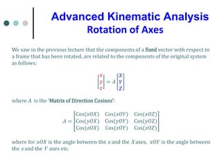
1. We saw in the previous lecture that the components of a fixed vector with respect to
a frame that has been rotated, are related to the components of the original system
as follows:
𝑥𝑥
𝑦𝑦
𝑧𝑧
= 𝐴𝐴
𝑋𝑋
𝑌𝑌
𝑍𝑍
where 𝐴𝐴 is the ‘Matrix of Direction Cosines’:
𝐴𝐴 =
Cos(𝑥𝑥𝑥𝑥𝑥𝑥) Cos(𝑥𝑥𝑥𝑥𝑥𝑥) Cos(𝑥𝑥𝑥𝑥𝑥𝑥)
Cos(𝑦𝑦𝑦𝑦𝑦𝑦) Cos(𝑦𝑦𝑦𝑦𝑦𝑦) Cos(𝑦𝑦𝑦𝑦𝑦𝑦)
Cos(𝑧𝑧𝑧𝑧𝑧𝑧) Cos(𝑧𝑧𝑧𝑧𝑧𝑧) Cos(𝑧𝑧𝑧𝑧𝑧𝑧)
where for 𝑥𝑥𝑥𝑥𝑥𝑥 is the angle between the x and the X axes, 𝑥𝑥𝑥𝑥𝑥𝑥 is the angle between
the x and the Y axes etc.
Rotation of Axes
Advanced Kinematic Analysis

2. We will now prove this from geometry.
X
Y
y x
A 2D Rotation
We also saw that the transformation for a 2D rotation about the z axis
simplifies to:
𝑥𝑥
𝑦𝑦
𝑧𝑧
=
Cos(𝑥𝑥𝑥𝑥𝑥𝑥) Cos(𝑥𝑥𝑥𝑥𝑥𝑥) 0
Cos(𝑦𝑦𝑦𝑦𝑦𝑦) Cos(𝑦𝑦𝑦𝑦𝑦𝑦) 0
0 0 1
𝑋𝑋
𝑌𝑌
𝑍𝑍
=
𝐶𝐶𝐶𝐶𝐶𝐶𝐶𝐶 𝑆𝑆𝑆𝑆𝑆𝑆𝑆𝑆 0
−𝑆𝑆𝑆𝑆𝑆𝑆𝑆𝑆 𝐶𝐶𝐶𝐶𝐶𝐶𝐶𝐶 0
0 0 1
𝑋𝑋
𝑌𝑌
𝑍𝑍
i.e.:
𝑥𝑥
𝑦𝑦 =
𝐶𝐶𝐶𝐶𝐶𝐶𝐶𝐶 𝑆𝑆𝑆𝑆𝑆𝑆𝑆𝑆
−𝑆𝑆𝑆𝑆𝑆𝑆𝑆𝑆 𝐶𝐶𝐶𝐶𝐶𝐶𝐶𝐶
𝑋𝑋
𝑌𝑌
Advanced Kinematic Analysis

3. Advanced Kinematic Analysis
2D Transformation - proof from geometry.
A 2D Rotation
Y
X
y
Y
X
y
x
And from the figure (using similar triangles) it is therefore evident that:
𝑥𝑥
𝑦𝑦 =
cos 𝜃𝜃 sin 𝜃𝜃
− sin 𝜃𝜃 cos 𝜃𝜃
𝑋𝑋
𝑌𝑌
end of proof
x

4. Advanced Kinematic Analysis
3D rotation of axes achieved by 3 successive 2D rotations
In general, we can always achieve any 3D rotation by 3 successive 2D rotations
(about the appropriate axes using the appropriate (3 x 3) 2D rotation matrix of
Direction Cosines) i.e.
i.e. 𝑥𝑥′ = 𝐴𝐴𝑋𝑋 ⟹ 𝑥𝑥′′ = 𝐴𝐴′𝑥𝑥′ ⟹ 𝑥𝑥′′′ = 𝐴𝐴′′𝑥𝑥′′
where the direction cosine matrices in each case (𝐴𝐴, 𝐴𝐴′
, and 𝐴𝐴′′
) are 2D
rotations about corresponding axes.
Orthogonality of matrix A
𝐴𝐴𝑇𝑇 = 𝐴𝐴−1 𝑖𝑖. 𝑒𝑒. 𝐴𝐴𝑇𝑇𝐴𝐴 = 𝐼𝐼 (the unit matrix)

5. Advanced Kinematic Analysis
A Physical rotation
A physical rotation can be obtained by keeping the axes fixed but rotating a
vector. Consider a point P on a disc. If the disc is rotated through angle θ,
the new position vector P* can be obtained by multiplying vector P by 𝐴𝐴−1
e.g.: Y
X
P
P*
i.e.
𝑃𝑃∗ = 𝐴𝐴−1𝑃𝑃 =
cos 𝜃𝜃 − sin 𝜃𝜃
sin 𝜃𝜃 cos 𝜃𝜃
𝑃𝑃𝑥𝑥
𝑃𝑃𝑦𝑦

6. Advanced Kinematic Analysis
KINEMATICS OF A PARTICLE OBTAINED BY ROTATION OF AXES
Here we return to the original task, namely the development of tools that
enable us to obtain the derivatives of vectors (particularly velocity and
acceleration) when the position vector is described in terms of a frame of
reference that is moving (i.e. a rotating frame). To do this, we initially
approach the problem in a ‘sledge-hammer’ way by rotation of axes (which,
from the previous section, we now know how to do).

7. Advanced Kinematic Analysis
KINEMATICS OF A PARTICLE OBTAINED BY ROTATION OF AXES
Consider a particle P, with position vector r, that is moving arbitrarily in the (fixed) XY
plane as described in the following figure where P’ is a new position. Here the particle is
‘tracked’ by a frame of reference xy such that the x axis always points straight at the
particle. The xy axes are therefore moving polar coordinates. The question is: what are
the absolute velocity and acceleration vector for particle P? We will answer this
question using a rotation of axes.
P
X
Y
y
P’
x
r
P moves anyway in
the plane
P’ is a new position
Particle P moving arbitrarily in the XY Plane (where the XY frame is fixed). In addition, a (polar)
coordinate system xy is chosen as a special case to track particle P - the xy frame is therefore
moving.

8. Advanced Kinematic Analysis
KINEMATICS OF A PARTICLE OBTAINED BY ROTATION OF AXES
The position vector
Note the position vector 𝑟𝑟 of P is:
𝑟𝑟 = 𝑋𝑋 𝑡𝑡 𝐼𝐼 + 𝑌𝑌 𝑡𝑡 𝐽𝐽 = 𝑟𝑟 𝑡𝑡 cos 𝜃𝜃 𝑡𝑡 𝐼𝐼 + 𝑟𝑟 𝑡𝑡 sin 𝜃𝜃(𝑡𝑡)𝐽𝐽 𝐼𝐼 𝑎𝑎𝑎𝑎𝑎𝑎 𝐽𝐽 𝑓𝑓𝑓𝑓𝑓𝑓𝑓𝑓𝑓𝑓
The velocity vector
The velocity vector can be obtained by differentiation of the position vector with respect
to the fixed frame of reference, i.e.:
𝑉𝑉 = ̇
𝑟𝑟 =
𝑑𝑑
𝑑𝑑𝑑𝑑
𝑟𝑟 cos 𝜃𝜃 𝐼𝐼 + 𝑟𝑟 sin 𝜃𝜃 𝐽𝐽 = ̇
𝑟𝑟 cos 𝜃𝜃 − 𝑟𝑟 sin 𝜃𝜃 ̇
𝜃𝜃 𝐼𝐼 + ̇
𝑟𝑟 sin 𝜃𝜃 + 𝑟𝑟 cos 𝜃𝜃 ̇
𝜃𝜃 𝐽𝐽
(i.e. in the fixed system)

9. Advanced Kinematic Analysis
KINEMATICS OF A PARTICLE OBTAINED BY ROTATION OF AXES
The acceleration vector
The acceleration vector can be obtained again by differentiation of the velocity
vector with respect to the fixed frame of reference, i.e.:
𝑎𝑎 = ̈
𝑟𝑟 = ̈
𝑋𝑋𝐼𝐼 + ̈
𝑌𝑌𝐽𝐽
= ̈
𝑟𝑟 cos 𝜃𝜃 − ̇
𝑟𝑟 sin 𝜃𝜃 ̇
𝜃𝜃 − ̇
𝑟𝑟 sin 𝜃𝜃 ̇
𝜃𝜃 − 𝑟𝑟 cos 𝜃𝜃 ̇
𝜃𝜃2 − 𝑟𝑟 sin 𝜃𝜃 ̈
𝜃𝜃 𝐼𝐼
+ ̈
𝑟𝑟 sin 𝜃𝜃 + ̇
𝑟𝑟 cos 𝜃𝜃 ̇
𝜃𝜃 + ̇
𝑟𝑟 cos 𝜃𝜃 ̇
𝜃𝜃 + 𝑟𝑟 cos 𝜃𝜃 ̈
𝜃𝜃 − 𝑟𝑟 sin 𝜃𝜃 ̇
𝜃𝜃2 𝐽𝐽
(i.e. again in the fixed system)

10. Advanced Kinematic Analysis
KINEMATICS OF A PARTICLE OBTAINED BY ROTATION OF AXES
The position, velocity, and acceleration vectors in the moving system
The components of the position vector 𝑟𝑟 in the moving (polar) system can be obtained
by a 2D rotation matrix i.e.:
𝑥𝑥
𝑦𝑦 =
cos 𝜃𝜃 sin 𝜃𝜃
− sin 𝜃𝜃 cos 𝜃𝜃
𝑋𝑋(𝑡𝑡)
𝑌𝑌(𝑡𝑡)
i.e. since 𝑟𝑟 = 𝑋𝑋 𝑡𝑡 𝐼𝐼 + 𝑌𝑌 𝑡𝑡 𝐽𝐽 = 𝑟𝑟 𝑡𝑡 cos 𝜃𝜃 𝑡𝑡 𝐼𝐼 + 𝑟𝑟 𝑡𝑡 sin 𝜃𝜃(𝑡𝑡)𝐽𝐽 :
𝑥𝑥
𝑦𝑦 =
cos 𝜃𝜃 sin 𝜃𝜃
− sin 𝜃𝜃 cos 𝜃𝜃
𝑟𝑟 cos 𝜃𝜃
𝑟𝑟 sin 𝜃𝜃
And by noting that 𝑐𝑐𝑐𝑐𝑐𝑐2𝜃𝜃 + 𝑠𝑠𝑠𝑠𝑠𝑠2𝜃𝜃 = 1, we get:
𝑥𝑥
𝑦𝑦 =
𝑟𝑟
0
i.e. 𝑟𝑟 = 𝑟𝑟𝑖𝑖 (where 𝑖𝑖 is moving with angular velocity ̇
𝜃𝜃).
This result is obvious because the x axis always points straight at the particle so the
frame of reference xy (polar coordinates) is defined precisely to ‘track’ the particle.

11. Advanced Kinematic Analysis
The Velocity vector 𝑉𝑉 in the moving system
The components of the velocity vector obtained by a 2D rotation matrix i.e.:
𝑉𝑉 = ̇
𝑋𝑋𝐼𝐼 + ̇
𝑌𝑌𝐽𝐽 = ̇
𝑟𝑟 cos 𝜃𝜃 − 𝑟𝑟 sin 𝜃𝜃 ̇
𝜃𝜃 𝐼𝐼 + ̇
𝑟𝑟 sin 𝜃𝜃 + 𝑟𝑟 cos 𝜃𝜃 ̇
𝜃𝜃 𝐽𝐽
̇
𝑥𝑥
̇
𝑦𝑦
=
cos 𝜃𝜃 sin 𝜃𝜃
− sin 𝜃𝜃 cos 𝜃𝜃
̇
𝑋𝑋
̇
𝑌𝑌
=
̇
𝑟𝑟
𝑟𝑟 ̇
𝜃𝜃
i.e. the velocity vector in the moving system is:
̇
𝑟𝑟 = ̇
𝑟𝑟𝑖𝑖 + 𝑟𝑟 ̇
𝜃𝜃𝑗𝑗
KINEMATICS OF A PARTICLE OBTAINED BY ROTATION OF AXES

12. Advanced Kinematic Analysis
KINEMATICS OF A PARTICLE OBTAINED BY ROTATION OF AXES
Acceleration vector 𝒂𝒂 in the moving system
The components of the acceleration vector also obtained by a 2D rotation matrix are:
𝑎𝑎 = ̈
𝑋𝑋𝐼𝐼 + ̈
𝑌𝑌𝐽𝐽 = ̈
𝑟𝑟 cos 𝜃𝜃 − ̇
𝑟𝑟 sin 𝜃𝜃 ̇
𝜃𝜃 − ̇
𝑟𝑟 sin 𝜃𝜃 ̇
𝜃𝜃 − 𝑟𝑟 cos 𝜃𝜃 ̇
𝜃𝜃2
− 𝑟𝑟 sin 𝜃𝜃 ̈
𝜃𝜃 𝐼𝐼
+ ̈
𝑟𝑟 sin 𝜃𝜃 + ̇
𝑟𝑟 cos 𝜃𝜃 ̇
𝜃𝜃 + ̇
𝑟𝑟 cos 𝜃𝜃 ̇
𝜃𝜃 + 𝑟𝑟 cos 𝜃𝜃 ̈
𝜃𝜃 − 𝑟𝑟 sin 𝜃𝜃 ̇
𝜃𝜃2 𝐽𝐽
And in terms of the xy frame:
̈
𝑥𝑥
̈
𝑦𝑦
=
cos 𝜃𝜃 sin 𝜃𝜃
− sin 𝜃𝜃 cos 𝜃𝜃
̈
𝑋𝑋
̈
𝑌𝑌
And after some manipulation we get:
= ̈
𝑟𝑟 − 𝑟𝑟 ̇
𝜃𝜃2
2 ̇
𝑟𝑟 ̇
𝜃𝜃 + 𝑟𝑟 ̈
𝜃𝜃
i.e. the acceleration vector in the moving system is:
𝑎𝑎 = ( ̈
𝑟𝑟 − 𝑟𝑟 ̇
𝜃𝜃2)𝑖𝑖 + (2 ̇
𝑟𝑟 ̇
𝜃𝜃 + 𝑟𝑟 ̈
𝜃𝜃)𝑗𝑗

13. Advanced Kinematic Analysis
Physical Interpretation of Acceleration Terms
The components of the acceleration vector are now shown in the figure below where the
unit vectors 𝑖𝑖 , 𝑗𝑗 are moving.
P
X
Y
y
x
r=ri
r
̈
𝑟𝑟: is the radial acceleration.
−𝑟𝑟 ̇
𝜃𝜃2: is the centripetal acceleration.
𝑟𝑟 ̈
𝜃𝜃: is the tangential acceleration.
2 ̇
𝑟𝑟 ̇
𝜃𝜃: is the coriolis component.

14. Advanced Kinematic Analysis
The Coriolis acceleration stems from the combined radial and angular motion.
Imagine moving radially outwards on a spinning disc (e.g. a carousel or roundabout)
with constant angular velocity ω. At radius r1, the tangential velocity is v1= ωr1. At
radius r2, the tangential velocity is v2= ωr2. Since r2 > r1 the tangential velocity must
increase, representing an acceleration component in the tangential direction.
ωr1
𝑟𝑟2 > 𝑟𝑟1
̇
𝜃𝜃 = 𝜔𝜔 ̇
𝜔𝜔 = 0
ωr2
r1 r2