Hypothesis Testing Hypothesis The formal testing of hypothesis is a critical step not to be ignored. One of the jobs of statistics is to reduce the uncertainty in our decision making. It does so by helping to identify assumptions and check the validity, in essence, what is really there. It is my personal preference to evaluate stocks or mutual funds to see if they actually exceed the average market return of 10%. The 10% return is the historical return on stocks over the past 75 years, however, each year has its own unique return. When doing so, I am interested in did this mutual fund exceed the 10% annual return. When you look at hypothesis testing there are three ways you can set them up. There are as follows: HO: = H1: not equal Word In story problem: Is Different Ho: < or = H1: is greater than Word In story problem: more than, increased HO: > or = H1: Is less than Word In story problem: decreased, dropped The hypothesis come in “pre-packaged sets” so you can’t mix and match. So when you are setting them up, look at the alternative (H1) in setting them up. Many times this is the decision that interests you the most. In this case, I wanted returns that exceeded ten percent, so I looked at the alternative hypothesis of greater than when setting up the process. What is helpful in thinking about the hypothesis and alternative hypothesis are the unique qualities of the null or HO, hypotheses. The HO hypothesis has unique characteristics. The unique characteristics is that you assume there to either be “no difference” or status quo. So, I set the hypothesis up as follows: HO: return is less than or equal to ten percent H1: return is greater than ten percent For the hypothesis test, I could have chosen to have it set up two other ways and those are: HO: the return is equal to ten percent H1; the return is not equal to ten percent HO: The return is greater than or equal to ten percent H1: The return is less than ten percent. What is helpful in thinking about the hypothesis and alternative hypothesis are the unique qualities of the null or HO, hypotheses. The HO hypothesis has unique characteristics. The unique characteristics are that you assume there to either “no difference” or status quo. In the stating of HO there is always an implied equal. To help you understand this concept lets take a trip to the local vending machine. Hypothesis Test Thinking and a Vending Machine Imagine yourself walking up to a vending machine. You want to purchase a bottle of Pepsi for a $1.00. You walk up to the vending machine and assume you are going to put your dollar in the machine, press the Pepsi button, and the machine will dispense the bottle of Pepsi. Do you walk up to the machine, knowing that it is not going to give you your bottle of Pepsi after you insert your dollar? If so, would you proceed with the transaction. No you wouldn’t make the transaction and willingly lose your doll.

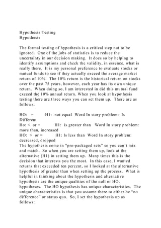
1. Hypothesis Testing
Hypothesis
The formal testing of hypothesis is a critical step not to be
ignored. One of the jobs of statistics is to reduce the
uncertainty in our decision making. It does so by helping to
identify assumptions and check the validity, in essence, what is
really there. It is my personal preference to evaluate stocks or
mutual funds to see if they actually exceed the average market
return of 10%. The 10% return is the historical return on stocks
over the past 75 years, however, each year has its own unique
return. When doing so, I am interested in did this mutual fund
exceed the 10% annual return. When you look at hypothesis
testing there are three ways you can set them up. There are as
follows:
HO: = H1: not equal Word In story problem: Is
Different
Ho: < or = H1: is greater than Word In story problem:
more than, increased
HO: > or = H1: Is less than Word In story problem:
decreased, dropped
The hypothesis come in “pre-packaged sets” so you can’t mix
and match. So when you are setting them up, look at the
alternative (H1) in setting them up. Many times this is the
decision that interests you the most. In this case, I wanted
returns that exceeded ten percent, so I looked at the alternative
hypothesis of greater than when setting up the process. What is
helpful in thinking about the hypothesis and alternative
hypothesis are the unique qualities of the null or HO,
hypotheses. The HO hypothesis has unique characteristics. The
unique characteristics is that you assume there to either be “no
difference” or status quo. So, I set the hypothesis up as
follows:

2. HO: return is less than or equal to ten percent
H1: return is greater than ten percent
For the hypothesis test, I could have chosen to have it set up
two other ways and those are:
HO: the return is equal to ten percent
H1; the return is not equal to ten percent
HO: The return is greater than or equal to ten percent
H1: The return is less than ten percent.
What is helpful in thinking about the hypothesis and alternative
hypothesis are the unique qualities of the null or HO,
hypotheses. The HO hypothesis has unique characteristics. The
unique characteristics are that you assume there to either “no
difference” or status quo. In the stating of HO there is always
an implied equal. To help you understand this concept lets take
a trip to the local vending machine.
Hypothesis Test Thinking and a Vending Machine
Imagine yourself walking up to a vending machine. You want
to purchase a bottle of Pepsi for a $1.00. You walk up to the
vending machine and assume you are going to put your dollar in
the machine, press the Pepsi button, and the machine will
dispense the bottle of Pepsi. Do you walk up to the machine,
knowing that it is not going to give you your bottle of Pepsi
after you insert your dollar? If so, would you proceed with the
transaction. No you wouldn’t make the transaction and
willingly lose your dollar. You assume that as you approach the
machine and put your money in that you will receive your Pepsi
because that is what has happened time after time, this is the
“status quo” segment of the hypothesis. Now, when the
machine doesn’t give you your Pepsi but keeps your dollar, you

3. REJECT the hypothesis that this machine is fair and ACCEPT
the alternative hypotheses that this machine has stolen my
money and is a crooked machine. Now that you know about the
formal hypothesis, let’s look at the rest of the procedure to
separate fact from fiction.
Remaining Hypothesis Testing Steps
Decision Rule:
The remaining steps are to set up the rules and check our
results. We set our rules up ahead of time so as not to be
unduly influenced by the results. So, we decide on a level of
significance. This is a significant level because it determines
the point at which we either accept or reject our null hypothesis.
The levels are normally.10, .05 or .01. These are similar to
purchasing a Pepsi in a small, medium or large, sorry; we don’t
have a super size in statistics. When choosing the levels of
significance, one can look at industry norm or you can choose
any one of the three. Normally, the .05 level of significance is
chosen because this is middle ground. So we chose the .05
level of significance.
Test Statistic
The next step is to calculate our “test statistic”. This is the
statistic that our computer software generates for us. This is
most easily expressed in probability or what is normally called
the “P” value. The “P” stands for probability and can be
thought of this way. If the “true average”, the average that is
really there, not our sample results, the probability of getting a
sample average which we found, is some value. Lets say that
we were testing the hypothesis that our mutual fund return is
less than or equal to ten percent and we input our data, test the
hypothesis at the .05 level of significance. The computer
software calculates a “P value” of .15. A .15 value is greater

4. than the .05 level of significance and so we don’t reject our
hypothesis and conclude the stock we are looking at has a return
less than or equal to 10%. However, if the “ P value”
calculated from the computer program was .04; we would have
rejected the null hypothesis and concluded that the average
return of this mutual fund was greater than ten percent.
Side Note: if the “P or probability value calculated “is less than
the level of significance, we reject the null hypothesis and
accept the alternative. We do this because we are saying that if
the null hypothesis is true, the probability of getting a sample
average with this result is less than the decision rule statistic.
Decision:
The decision is where you compare the probability value
calculated against the critical probability value set in your
decision rule. If your test probability value is less than the
critical, reject the null hypothesis and accept the alternative
hypothesis. The P value testing allows for you to be slightly
confident, if is just on the border line of accept or reject to very
confident if the probability value is very small such as .001
(1/1000)
You may need to double check your values and if unsure, you
can ask yourself do I want a 5% raise or do I want a .1% raise.
This is a simple way of keeping your decision correct and not
confusing the decision because you misinterpreted the p values
size.
Traditional Approach
In 2004, a small dealership leased 21 Chevrolet Impalas on two
year leases. When the cars were returned in 2006, the mileage
recorded was (see table). Is the dealers mean significantly
greater than the national average of 30,000 miles for two year

5. leased vehicles at the 10% level of significance?
T value = 21-1 = 20 , one tailed test, .10 level of significance
= 1.325
HO: The average miles is less than or equal to 30,000
H1: The average miles are greater than 30,000
Decision Rule: If the T value calculated is greater than 1.325,
reject HO
Test Statistic: T= ( 33,950-30,000)/ (11,866/√21)
= ( 33,950-30,000)/ (11,866/4.58)
= 3,950/ 2,590
T value =1.52
Decision: Since the Test statistic of 1.52 is greater than the T
critical value of 1.325, we reject HO and conclude the cars have
more mileage.
EMBED MtbGraph.Document.15
0
.
4
0
.
3
0
.
2
0
.
1

6. 0
.
0
X
D
e
n
s
i
t
y
D
i
s
t
r
i
b
u
t
i
o
n
P
l
o
t
N
o
r
m
a
l
,

7. M
e
a
n
=
0
,
S
t
D
e
v
=
1
6
0
0
0
0
5
0
0
0
0
4
0
0
0
0
3
0
0

8. 0
0
2
0
0
0
0
M
e
d
i
a
n
M
e
a
n
4
0
0
0
0
3
5
0
0
0
3
0
0
0
0
2
5
0
0

9. 0
1
s
t
Q
u
a
r
t
i
l
e
2
4
6
1
5
M
e
d
i
a
n
3
3
3
8
0
3
r
d
Q
u
a

10. r
t
i
l
e
4
3
4
4
5
M
a
x
i
m
u
m
5
8
6
3
0
2
8
5
4
8
3
9
3
5
1
2
5
0
4

11. 8
4
2
2
7
5
9
0
7
8
1
7
1
3
6
A
-
S
q
u
a
r
e
d
0
.
2
8
P
-
V
a
l
u
e
0

12. .
5
9
5
M
e
a
n
3
3
9
5
0
S
t
D
e
v
1
1
8
6
6
V
a
r
i
a
n
c
e
1
4
0
8
0

13. 6
0
8
5
S
k
e
w
n
e
s
s
0
.
2
9
3
7
1
9
K
u
r
t
o
s
i
s
-
0
.
5
5
7
0
3

14. 1
N
2
1
M
i
n
i
m
u
m
1
4
3
1
0
A
n
d
e
r
s
o
n
-
D
a
r
l
i
n
g
N
o
r

15. m
a
l
i
t
y
T
e
s
t
9
5
%
C
o
n
f
i
d
e
n
c
e
I
n
t
e
r
v
a
l
f

16. o
r
M
e
a
n
9
5
%
C
o
n
f
i
d
e
n
c
e
I
n
t
e
r
v
a
l
f
o
r
M

17. e
d
i
a
n
9
5
%
C
o
n
f
i
d
e
n
c
e
I
n
t
e
r
v
a
l
f
o
r
S
t
D

18. e
v
9
5
%
C
o
n
f
i
d
e
n
c
e
I
n
t
e
r
v
a
l
s
S
u
m
m
a
r
y
f
o

19. r
M
i
l
e
a
g
e
P value Approach
HO: The average miles is less than or equal to 30,000
H1: The average miles are greater than 30,000
Decision Rule: If the P value calculated is less than .10, reject
HO
Test Statistic: .071
Decision: Since the Test statistic of .071 is less than the P
critical value of .10, we reject HO and have weak evidence to
conclude the cars have more mileage. For if the HO was true
that the cars had less than or equal to 30,000 miles, the
probability that you would have randomly found a sample
average of 33,950 is 7.1%, therefore, it is possible but not
probable.
6
0
0
0
0
5
0
0
0
0

20. 4
0
0
0
0
3
0
0
0
0
2
0
0
0
0
1
0
0
0
0
X
_
H
o
M
i
l
e
a
g
e
B
o
x
p
l

21. o
t
o
f
M
i
l
e
a
g
e
(
w
i
t
h
H
o
a
n
d
9
5
%
t
-
c
o
n
f

22. i
d
e
n
c
e
i
n
t
e
r
v
a
l
f
o
r
t
h
e
m
e
a
n
)
Box Plot Explanation: The red HO circle is the null hypothesis
value. The blue line is the confidence interval and the xbar is
the sample average from which a 90% confidence interval was
created. Since the HO value is contained in the confidence
interval, it is possible that it could be the “real mean”.

23. Data
40,060
24,960
14,310
17,370
44,740
44,550
20,250
33,380
24,270
41,740
58,630
35,830
25,750
28,910
25,090
43,380
23,940
43,510
53,680
31,810
36,780
Traditional Method
Investment Company of America
8
0
6
0
4
0
2
0

24. 0
-
2
0
-
4
0
M
e
d
i
a
n
M
e
a
n
2
0
1
8
1
6
1
4
1
2
1
0
1
s
t
Q
u
a

25. r
t
i
l
e
0
.
9
0
0
M
e
d
i
a
n
1
6
.
3
0
0
3
r
d
Q
u
a
r
t
i
l
e
2
6

26. .
3
0
0
M
a
x
i
m
u
m
8
3
.
1
0
0
1
0
.
1
0
2
1
8
.
9
3
9
1
0
.
5
0
4
1

27. 9
.
8
0
0
1
6
.
0
2
2
2
2
.
3
6
7
A
-
S
q
u
a
r
e
d
0
.
5
1
P
-
V
a
l
u

28. e
0
.
1
8
6
M
e
a
n
1
4
.
5
2
0
S
t
D
e
v
1
8
.
6
6
8
V
a
r
i
a
n
c
e
3

29. 4
8
.
4
7
7
S
k
e
w
n
e
s
s
0
.
3
8
5
0
9
K
u
r
t
o
s
i
s
2
.
1
5
1
9
4

30. N
7
1
M
i
n
i
m
u
m
-
3
8
.
5
0
0
A
n
d
e
r
s
o
n
-
D
a
r
l
i
n
g
N
o

31. r
m
a
l
i
t
y
T
e
s
t
9
5
%
C
o
n
f
i
d
e
n
c
e
I
n
t
e
r
v
a
l

32. f
o
r
M
e
a
n
9
5
%
C
o
n
f
i
d
e
n
c
e
I
n
t
e
r
v
a
l
f
o
r

33. M
e
d
i
a
n
9
5
%
C
o
n
f
i
d
e
n
c
e
I
n
t
e
r
v
a
l
f
o
r
S
t

34. D
e
v
9
5
%
C
o
n
f
i
d
e
n
c
e
I
n
t
e
r
v
a
l
s
S
u
m
m
a
r
y
f

35. o
r
I
n
v
e
s
t
m
e
n
t
C
o
m
p
a
n
y
o
f
A
m
e
r
i
c
a
R
e
One Mutual Fund Scenario

36. .05 Level of Significance
HO: The average return on the Investment Company of
America is equal to 10%
H1: The average return on the Investment Company of America
is not equal to 10%
Decision Rule: If the Z value is less than -1.96 or greater than
1.96, reject HO
Test Statistic: Z = (14.52 – 10)/(18.668/√71)
Z = 4.52/2.21
Z = 2.04
Decision: Since the the Z value calculated of 2.04 is greater
than the Z critical of 1.96 we reject HO and conclude the fund
annual return is different than 10%
Since this was a two tailed test, the .05 reject region was
divided equally on both sides, thus is gives a .025 rejection
zone on each side. Since 50% probability is on each side of the
bell curve, we calculate the z value by 50% - 2.5% = 47.5%
.4750 = Z value of 1.96
NOTES:
2.21 is the standard error of the mean, when the standard
deviation is adjusted to reflect sample size based upon the
theory of the law of large numbers that as sample size increases,
variation decreases.

37. 0
.
4
0
.
3
0
.
2
0
.
1
0
.
0
X
D
e
n
s
i
t
y
D
i
s
t
r
i
b
u
t
i
o
n

38. P
l
o
t
N
o
r
m
a
l
,
M
e
a
n
=
0
,
S
t
D
e
v
=
1
Suppose we are interested now in does the fund beat the
historical average of 10%. It will take the following steps.
Note: This is a one tailed test and you need to remember which
is the positive side and negative side of the bell curvewith Left
is negative, right is positive
HO: The average return on the Investment Company of

39. America is less than or equal to 10%
H1: The average return on the Investment Company of America
is greater than 10%
Decision Rule: If the Z value is greater than Z 1.65, reject HO
Test Statistic: Z = (14.52 – 10)/(18.668/√71)
Z = 4.52/2.21
Z = 2.04
Decision: Since the the Z value calculated of 2.04 is greater
than the Z critical of 1.65,we reject HO and conclude the fund
annual return is greater than 10%
Since this was a one tailed test, the .05 reject region is located
on one side of the bell curve, thus to gain a Z value we subtract
our level of significance, in this case .05 thus 50% - 5% = 455%
.45 = Z value of 1.645
0
.
4
0
.
3
0
.
2
0
.

40. 1
0
.
0
X
D
e
n
s
i
t
y
D
i
s
t
r
i
b
u
t
i
o
n
P
l
o
t
N
o
r
m
a
l
,

41. M
e
a
n
=
0
,
S
t
D
e
v
=
1
Suppose we are interested now in does the fund less the
historical average of 10%. It will take the following steps.
HO: The average return on the Investment Company of
America is greater than or equal to 10%
H1: The average return on the Investment Company of America
is less than 10%
Decision Rule: If the Z value is less than Z -1.65, reject HO
Test Statistic: Z = (14.52 – 10)/(18.668/√71)
Z = 4.52/2.21
Z = 2.04
Decision: Since the the Z value calculated of 2.04 is greater

42. than the Z critical of
- 1.65,we fail reject HO and conclude the fund annual return is
greater than or equal to 10%
0
.
4
0
.
3
0
.
2
0
.
1
0
.
0
X
D
e
n
s
i
t
y
D
i
s
t
r
i

43. b
u
t
i
o
n
P
l
o
t
N
o
r
m
a
l
,
M
e
a
n
=
0
,
S
t
D
e
v
=
1
P Value Approach

44. The formal steps look like this:
One Mutual Fund Scenario
One-Sample Z: Investment Company of America
Test of mu = 10 vs not = 10
The assumed standard deviation = 18.668
Variable N Mean StDev SE Mean 95% CI
Z
Investment Company of Am 71 14.52 18.67 2.22 (10.18,
18.86) 2.04
Variable P
Investment Company of Am 0.041
HO: The average return on the Investment Company of
America is equal to 10%
H1; The average return of the Investment Company of America
of is not equal to 10%
Decision Rule: If the P value is less than .05 reject the HO
Test Statistic: .041
Decision: Since the probability statistics calculated of .041 is
less than the critical probability value of .05, we reject the null
hypothesis and are somewhat confident that the return on this
fund is not equal to 10%. For if the HO was true that the funds
real average is10%, the probability that you would have

45. randomly found a sample average of 14.51 is 4.1%, therefore, it
is possible but not probable
NOTES
One-Sample Z: Investment Company of America
Test of mu = 10 vs > 10
The assumed standard deviation = 18.668
95% Lower
Variable N Mean StDev SE Mean Bound Z
P
Investment Company of Am 71 14.52 18.67 2.22 10.88
2.04 0.021
Suppose we are interested now in does the fund beat the
historical average of 10%. It will take the following steps.
HO: The average return on the Investment Company of
America is less than or equal to 10%
H1: The average return on the Investment Company of America
is greater than 10%
Decision Rule: If the P value calculate is less than .05, reject
HO
Test Statistic: .021
Decision: Since the probability statistics calculated of .021 is
less than the critical probability value of .05, we reject the null
hypothesis and are somewhat confident that the return on this
fund is greater than 10%. For if the HO was true that the funds
real average is less than or equal to10%, the probability that

46. you would have randomly found a sample average of 14.51 is
2.1%, therefore, it is possible but not probable
NOTES
One-Sample Z: Investment Company of America
Test of mu = 10 vs < 10
The assumed standard deviation = 18.668
95% Upper
Variable N Mean StDev SE Mean Bound Z
P
Investment Company of Am 71 14.52 18.67 2.22 18.16
2.04 0.979
Suppose we are interested now in does the fund earns less than
the historical average of 10%. It will take the following steps.
HO: The average return on the Investment Company of
America is greater than or equal to 10%
H1: The average return on the Investment Company of America
is less than 10%
Decision Rule: If the P value calculate is less than .05, reject
HO
Test Statistic: .979
Decision: Since the probability statistics calculated of .979 is
greater than the critical probability value of .05, we fail to
reject the null hypothesis and are very confident that the return
on this fund is greater than or equal to 10%. For if the HO was
true that the funds real average is greater than or equal 10%, the

47. probability that you would have randomly found a sample
average of 14.51 is 97.9%, therefore, it is possible and
probable.
NOTES:
Hypothesis Testing Notes
E-Tickets
Most air traffic passenger use e-tickets. Electronic ticketing
allows passengers not worry about paper tickets and it reduces
the airlines costs. However in recent times airlines have begun
to receive complaints from passengers regarding e-tickets,
especially when having to switch planes. To investigate this
problem an independent watchdog agency contacted a random
sample of 21 airports and collected data on the number of
complaints due to e-tickets.
At the .05 level of significance is there evidence to conclude
that the ten year average of 15 complaints per month has now
changed and actually increased due to electronic ticketing?
Problem Statement:
HO:
H1
Decision Rule
Test Statistic:
Decision
NOTES
1
6
1

48. 5
1
4
1
3
1
2
1
1
1
0
M
e
d
i
a
n
M
e
a
n
1
4
.
5
0
1
4
.
2
5
1
4
.
0
0

49. 1
3
.
7
5
1
3
.
5
0
1
3
.
2
5
1
3
.
0
0
1
s
t
Q
u
a
r
t
i
l
e
1
2
.
5

50. 0
0
M
e
d
i
a
n
1
4
.
0
0
0
3
r
d
Q
u
a
r
t
i
l
e
1
5
.
0
0
0
M
a
x
i

51. m
u
m
1
6
.
0
0
0
1
2
.
8
8
8
1
4
.
2
5
5
1
3
.
0
0
0
1
4
.
3
2
6
1
.
1

52. 4
9
2
.
1
7
0
A
-
S
q
u
a
r
e
d
0
.
4
7
P
-
V
a
l
u
e
0
.
2
2
1
M
e
a
n

53. 1
3
.
5
7
1
S
t
D
e
v
1
.
5
0
2
V
a
r
i
a
n
c
e
2
.
2
5
7
S
k
e
w
n
e
s

54. s
-
0
.
3
4
7
2
1
7
K
u
r
t
o
s
i
s
0
.
1
2
4
0
6
6
N
2
1
M
i
n
i
m
u
m

55. 1
0
.
0
0
0
A
n
d
e
r
s
o
n
-
D
a
r
l
i
n
g
N
o
r
m
a
l
i
t
y
T
e
s

56. t
9
5
%
C
o
n
f
i
d
e
n
c
e
I
n
t
e
r
v
a
l
f
o
r
M
e
a
n
9
5
%

57. C
o
n
f
i
d
e
n
c
e
I
n
t
e
r
v
a
l
f
o
r
M
e
d
i
a
n
9
5
%
C

58. o
n
f
i
d
e
n
c
e
I
n
t
e
r
v
a
l
f
o
r
S
t
D
e
v
9
5
%
C
o
n
f

59. i
d
e
n
c
e
I
n
t
e
r
v
a
l
s
S
u
m
m
a
r
y
f
o
r
E
-
T
i
c
k
e
t

60. E-Tickets
Most air traffic passenger use e-tickets. Electronic ticketing
allows passengers not worry about paper tickets and it reduces
the airlines costs. However in recent times airlines have begun
to receive complaints from passengers regarding e-tickets,
especially when having to switch planes. To investigate this
problem an independent watchdog agency contacted a random
sample of 21 airports and collected data on the number of
complaints due to e-tickets.
At the .05 level of significance is there evidence to conclude
that the ten year average of 15 complaints per month has now
changed and actually increased due to electronic ticketing?
Problem Statement:
The airline industry has undergone significant changes
including the movement to e-tickets to reduce costs of paper
tickets as well as allow for internet booking and reservation.
However, given the tight markets and strong competition, the
airline knows it needs to minimize consumer complaints as this
translates into customer defection and loss of revenue.
T test is one tailed (.05) with sample size 21 – 1 = 20 degrees
of freedom = 1.725
HO: Complaints are less than or equal to 15
H1: Complaints are greater than 15
Decision Rule If T is > 1.725, reject HO
Test Statistic: Test Statistic: T = (13.751 – 15)/(1.502/√21)
T= -1.429/.3277

61. T = -4.36
Decision: Since T calculated of -4.36 is less than T critical of
1.725, we fail to reject HO.
0
.
4
0
.
3
0
.
2
0
.
1
0
.
0
X
D
e
n
s
i
t
y
D
i
s
t
r
i

62. b
u
t
i
o
n
P
l
o
t
N
o
r
m
a
l
,
M
e
a
n
=
0
,
S
t
D
e
v
=
1

63. E-Tickets
Most air traffic passenger use e-tickets. Electronic ticketing
allows passengers not worry about paper tickets and it reduces
the airlines costs. However in recent times airlines have begun
to receive complaints from passengers regarding e-tickets,
especially when having to switch planes. To investigate this
problem an independent watchdog agency contacted a random
sample of 21 airports and collected data on the number of
complaints due to e-tickets.
At the .05 level ofsignificance is there evidence to conclude that
the ten year average of 15 complaints per month has now
changed and actually increased due to electronic ticketing?
Problem Statement:
The airline industry has undergone significant changes
including the movement to e-tickets to reduce costs of paper
tickets as well as allow for internet booking and reservation.
However, given the tight markets and strong competition, the
airline knows it needs to minimize consumer complaints as this
translates into customer defection and loss of revenue.
HO: Complaints are less than or equal to 15
H1: Complaints are greater than 15
Decision Rule: If P calculated is less than .05, reject HO
Test Statistic: 1.00 actually is .9999 but was rounded up to one
Decision: Since the probability value calculated of .9999 is
greater than .05, we fail to reject HO and conclude there is
strong evidence to support that the number of complaints has
not increased. For if the HO was true that the funds real average
of complaints are less than or equal to 15, the probability that
you would have randomly found a sample average of 13.571 is

64. 99.9%, therefore, it is possible and very probable.
Test of mu = 15 vs > 15
95% Lower
Variable N Mean StDev SE Mean Bound T P
E-Ticket 21 13.571 1.502 0.328 13.006 -4.36 1.000
Chicken Feed
Raising chickens in commercial chicken farms is a growing
industry, as there is a shift from red meat to more white meat.
New Jersey Red Chickens are a favorite chicken and the Feed is
Us company has a new chicken food that they claim is excellent
for increasing weight and naturally it costs more. You have
heard this line before and therefore are skeptical but the
potential pay off is huge. You buy a small amount and feed it
to ten chickens, which you choose at random.
At the .01 level of significance is there evidence that the
chicken weight exceeds the average chicken weight of 4.35
pounds.
Problem Statement:
HO:
H1
Decision Rule
Test Statistic:
Decision
Notes:
4
.
4

65. 2
4
.
4
0
4
.
3
8
4
.
3
6
4
.
3
4
4
.
3
2
4
.
3
0
M
e
d
i
a
n
M
e
a
n
4

66. .
4
0
4
.
3
8
4
.
3
6
4
.
3
4
4
.
3
2
1
s
t
Q
u
a
r
t
i
l
e
4
.
3
4
5

67. 0
M
e
d
i
a
n
4
.
3
7
5
0
3
r
d
Q
u
a
r
t
i
l
e
4
.
3
9
2
5
M
a
x
i
m

68. u
m
4
.
4
1
0
0
4
.
3
3
3
1
4
.
4
0
2
9
4
.
3
2
5
9
4
.
4
0
1
4
0
.
0
2

69. 1
0
0
.
0
7
7
3
A
-
S
q
u
a
r
e
d
0
.
2
7
P
-
V
a
l
u
e
0
.
5
8
6
M
e
a

70. n
4
.
3
6
8
0
S
t
D
e
v
0
.
0
3
3
9
V
a
r
i
a
n
c
e
0
.
0
0
1
2
S
k
e
w

71. n
e
s
s
-
0
.
8
7
3
9
8
3
K
u
r
t
o
s
i
s
0
.
3
0
9
7
5
6
N
1
0
M
i
n
i

72. m
u
m
4
.
3
0
0
0
A
n
d
e
r
s
o
n
-
D
a
r
l
i
n
g
N
o
r
m
a
l
i
t
y

73. T
e
s
t
9
9
%
C
o
n
f
i
d
e
n
c
e
I
n
t
e
r
v
a
l
f
o
r
M
e
a
n

74. 9
9
%
C
o
n
f
i
d
e
n
c
e
I
n
t
e
r
v
a
l
f
o
r
M
e
d
i
a
n
9
9

75. %
C
o
n
f
i
d
e
n
c
e
I
n
t
e
r
v
a
l
f
o
r
S
t
D
e
v
9
9
%
C

76. o
n
f
i
d
e
n
c
e
I
n
t
e
r
v
a
l
s
S
u
m
m
a
r
y
f
o
r
C
h
i
c
k

77. e
n
W
e
i
g
h
t
s
Chicken Feed
Raising chickens in commercial chicken farms is a growing
industry, as there is a shift from red meat to more white meat.
New Jersey Red Chickens are a favorite chicken and the Feed is
Us company has a new chicken food that they claim is excellent
for increasing weight and naturally it costs more. You have
heard this line before and therefore are skeptical but the
potential pay off is huge. You buy a small amount and feed it
to ten chickens, which you choose at random.
At the .01 level of significance is there evidence that the
chicken weight exceeds the average chicken weight of 4.35
pounds.
Problem Statement:
HO: The chicken weight is less than or equal to 4.35 pounds
H1: The chicken weight is greater than 4.35 pounds
Decision Rule If T is > 2.821, reject HO
T test is one tailed (.01) with sample size 10 – 1 = 9 degrees of
freedom = 2.821
Test Statistic: Test Statistic: T = (4.368 – 4.35)/(.0339/√10)
T= .018/.0107

78. T = 1.68
Decision: Since T calculated of 1.68 is less than T critical of
2.821, we do not reject HO.
Notes:
0
.
4
0
.
3
0
.
2
0
.
1
0
.
0
X
D
e
n
s
i
t
y
D
i
s
t
r

79. i
b
u
t
i
o
n
P
l
o
t
N
o
r
m
a
l
,
M
e
a
n
=
0
,
S
t
D
e
v
=
1

80. Chicken Feed
Raising chickens in commercial chicken farms is a growing
industry, as there is a shift from red meat to more white meat.
New Jersey Red Chickens are a favorite chicken and the Feed is
Us company has a new chicken food that they claim is excellent
for increasing weight and naturally it costs more. You have
heard this line before and therefore are skeptical but the
potential pay off is huge. You buy a small amount and feed it
to ten chickens, which you choose at random.
At the .01 level of significance is there evidence that the
chicken weight exceeds the average chicken weight of 4.35
pounds.
Problem Statement:
HO: The chicken weight is less than or equal to 4.35 pounds
H1: The chicken weight is greater than 4.35 pounds
Decision Rule: If P calculated is less than .01, reject HO
Test Statistic: .064
Decision: Since the P value calculated of .064 is greater than
.01, we fail to reject HO and are only somewhat confident the
real chicken weight is less than or equal to 4.35 pounds For if
the HO was true that the real average chicken weigh is less than
or equal to 4.35, the probability that you would have randomly
found a sample average of 4.368 is 6.4%, therefore, it is
possible and probable.
Issue: small sample size, law of large numbers as sample size
increases variation decreases.
Test of mu = 4.35 vs > 4.35
Small sample law of large number
99% Lower
Variable N Mean StDev SE Mean Bound T P

81. Chicken Weights 10 4.3680 0.0339 0.0107 4.3377 1.68
0.064
4
.
4
2
4
.
4
0
4
.
3
8
4
.
3
6
4
.
3
4
4
.
3
2
4
.
3
0
X
_
H

82. o
C
h
i
c
k
e
n
W
e
i
g
h
t
s
B
o
x
p
l
o
t
o
f
C
h
i
c
k
e
n
W

83. e
i
g
h
t
s
(
w
i
t
h
H
o
a
n
d
9
9
%
t
-
c
o
n
f
i
d
e
n
c
e

84. i
n
t
e
r
v
a
l
f
o
r
t
h
e
m
e
a
n
)
Confidence interval contains the null hypothesis, so it is
possible it contains the real average.
Notes:
AARP Work Survey
The American Association of Retired Persons (AARP) reports
that 60% of retired persons under the age of 65 would be
willing to return to work on a full time basis if a suitable job
were available. A sample of 500 retired persons under the age
of 65 revealed 315 would return to work. At the .05 level of
significance can we conclude that more than 60% of retired
people in the age group would return to work?

85. Problem Statement:
In today’s economy, each person is responsible for their own
retirement investment decisions. Many retirees are forced to
return to work to pay bills since their retirement savings are
inadequate and there are also those who return to work for
socialization and wanting to continue to make contributions to
society. The question is today are more senior citizens
returning to work than in previous generations? This has
profound social and economic ramifications.
HO:
H1
Decision Rule
Test Statistic:
Decision
Notes:
AARP Work Survey
The American Association of Retired Persons (AARP) reports
that 60% of retired persons under the age of 65 would be
willing to return to work on a full time basis if a suitable job
were available. A sample of500 retired persons under the age
of 65 revealed 315 would return to work. At the .05 level of
significance can we conclude that more than60% of retired
people in the age group would return to work?
Problem Statement:
In today’s economy, each person is responsible for their own
retirement investment decisions. Many retirees are forced to
return to work to pay bills since their retirement savings are
inadequate and there are also those who return to work for
socialization and wanting to continue to make contributions to
society. The question is today are more senior citizens
returning to work than in previous generations? This has
profound social and economic ramifications.

86. Z value is used since it is a proportion
HO: The proportion of retired persons returning to work is less
than or equal to 60%
H1: The proportion of retired persons returning to work is
greater than 60%
Decision Rule: If z calculated is greater than 1.645, reject HO
Test Statistic: Z = .63-.60/ (√.63*.37/500)
Z = 1.38
315/500= .63
1-.63 = .37
Decision Since the Z calculated of 1.38 is less than the critical
value of 1.645, we fail to reject HO and conclude the average is
still less than or equal to 60%.
0
.
4
0
.
3
0
.
2
0
.
1
0
.
0
X

87. D
e
n
s
i
t
y
D
i
s
t
r
i
b
u
t
i
o
n
P
l
o
t
N
o
r
m
a
l
,
M
e
a
n

88. =
0
,
S
t
D
e
v
=
1
AARP Work Survey
The American Association of Retired Persons (AARP) reports
that 60% of retired persons under the age of 65 would be
willing to return to work on a full time basis if a suitable job
were available. A sample of 500 retired persons under the age
of 65 revealed 315 would return to work. . At the .05 level of
significance can we conclude that more than60% of retired
people in the age group would return to work?
Problem Statement:
In today’s economy, each person is responsible for their own
retirement investment decisions. Many retirees are forced to
return to work to pay bills since their retirement savings are
inadequate and there are also those who return to work for
socialization and wanting to continue to make contributions to
society. The question is today are more senior citizens
returning to work than in previous generations? This has
profound social and economic ramifications.
HO: The proportion of retired persons returning to work is less
than or equal to 60%
H1: The proportion of retired persons returning to work is
greater than 60%

89. Decision Rule: If P calculated is less than .05, reject HO
Test Statistic: .085
Decision: Since the P value calculated of .085 is greater than
.05, we fail to reject HO and are only somewhat confident the
real percentage of senior citizens returning to work is less than
or equal to 60%. For if the HO was true that the number of
people willing to return to work is less than or equal to 60%,
the probability that you would have randomly found a sample
average of 63% is 8.5%, therefore, it is possible and probable
AARP Work Survey
Test of p = 0.6 vs p > 0.6
95%
Lower
Sample X N Sample p Bound Z-Value P-Value
1 315 500 0.630000 0.594485 1.37 0.085
Hypothesis Test Directions for Minitab
Step One Sample Z Hypothesis Test
Begin by clicking on stat, basic stat then on One Sample Z
Step Two for Z Hypothesis Test
1. Click on the column of data to be used: Investment Company
of America
2. Enter the standard deviation value calculated from the
graphical summary of the data which is 18.66

90. 3. Click on perform hypothesis test
4. Enter the value for the test 10
5. Click on the Options Box
Step Three for Z Hypothesis Test
· Click on options
· Enter the alternative hypothesis test which in this example is
greater than
· Enter the confidence interval value that corresponds with the
level of significance in this example it is 95%
Step Four for Z Hypothesis Test
· Click on graphs
· Check the boxplot of data or other graph of your choosing.
· Click OK
Step Five for Z Hypothesis Test
Click OK to run the test
Step Six for Z Hypothesis Test
Results of the test
Results of the test are now showing in the session window and
you can copy and paste them into a graph or word document.

91. Directions for a One Sample T Test
Step 1
Enter your data and give them column headings for ease of use.
……..
Click on the menu and if you have a sample size smaller than 30
click on the one sample T or if your standard deviation is
calculated from your sample data, you will use a one sample T
test. One sample means you are only comparing one average
calculated from the of data against the historical or status quo
mean.
Step 2
Now that you have chosen the test, you will need to indicate
where the data is found by clicking on the column where the
data is located, unless you have what is called summarized data.
Summarized data is when you have already calculated or been
given the sample size, sample average and sample standard
deviation.
If your data is in a column such as the example, click the data
column heading to move it into the box.
If summarized data, where the mean, standard deviation and
sample size are given, then click on the “summarized data” dot
and enter the information into the boxes.
Step 3

92. · In this step you will need to check the hypothesis test box and
then
· Enter the value tested in this case it is 4.35 pounds.
· Click Options
Step 4
· Enter the confidence interval level that corresponds with the
level of significance. In this case our level of significance is
.05, so the corresponding level of significance is 95%
· Select the correct H1
· Click on OK
Step 5
· In this step you will choose the graph options that would be
most helpful to you. You can check all three and then look at
the options as they appear to decide which is most helpful. In
this case we choose a boxplot
· Click on boxplot
Step 6
Session Window with Results
· The hypothesis test listed with the alternative hypothesis
being referred to as the “vs not”.

93. · The P value associated with the hypothesis test and other
values are listed in the “”Variable output” section of this view.
Step 7
Graphical Analysis
4
.
4
2
4
.
4
0
4
.
3
8
4
.
3
6
4
.
3
4
4
.
3
2
4
.
3

94. 0
X
_
H
o
C
h
i
c
k
e
n
W
e
i
g
h
t
s
B
o
x
p
l
o
t
o
f
C
h
i
c
k

95. e
n
W
e
i
g
h
t
s
(
w
i
t
h
H
o
a
n
d
9
5
%
t
-
c
o
n
f
i
d
e

96. n
c
e
i
n
t
e
r
v
a
l
f
o
r
t
h
e
m
e
a
n
)
In graphical analysis you are looking to see if the HO is
contained in the confidence interval as if the confidence interval
is contained, you do not reject HO because it is possible that it
could be the “real average”.
Summarized Data
Step One ( if given, skip this step and go to step two)

97. 4
.
4
2
4
.
4
0
4
.
3
8
4
.
3
6
4
.
3
4
4
.
3
2
4
.
3
0
M
e
d
i
a
n
M

98. e
a
n
4
.
4
0
4
.
3
9
4
.
3
8
4
.
3
7
4
.
3
6
4
.
3
5
4
.
3
4
1
s
t
Q

99. u
a
r
t
i
l
e
4
.
3
4
5
0
M
e
d
i
a
n
4
.
3
7
5
0
3
r
d
Q
u
a
r
t
i
l

100. e
4
.
3
9
2
5
M
a
x
i
m
u
m
4
.
4
1
0
0
4
.
3
4
3
7
4
.
3
9
2
3
4
.
3
4

101. 3
2
4
.
3
9
3
4
0
.
0
2
3
3
0
.
0
6
1
9
A
-
S
q
u
a
r
e
d
0
.
2
7
P
-
V

102. a
l
u
e
0
.
5
8
6
M
e
a
n
4
.
3
6
8
0
S
t
D
e
v
0
.
0
3
3
9
V
a
r
i
a
n

103. c
e
0
.
0
0
1
2
S
k
e
w
n
e
s
s
-
0
.
8
7
3
9
8
3
K
u
r
t
o
s
i
s
0
.
3

104. 0
9
7
5
6
N
1
0
M
i
n
i
m
u
m
4
.
3
0
0
0
A
n
d
e
r
s
o
n
-
D
a
r
l
i
n

105. g
N
o
r
m
a
l
i
t
y
T
e
s
t
9
5
%
C
o
n
f
i
d
e
n
c
e
I
n
t
e
r

106. v
a
l
f
o
r
M
e
a
n
9
5
%
C
o
n
f
i
d
e
n
c
e
I
n
t
e
r
v
a
l

107. f
o
r
M
e
d
i
a
n
9
5
%
C
o
n
f
i
d
e
n
c
e
I
n
t
e
r
v
a
l
f
o

108. r
S
t
D
e
v
9
5
%
C
o
n
f
i
d
e
n
c
e
I
n
t
e
r
v
a
l
s
S
u
m
m
a

109. r
y
f
o
r
C
h
i
c
k
e
n
W
e
i
g
h
t
s
Prior to using summarized data you can find the information in
a graphical summary but most of the time it is given.
Step Two
Enter the sample size, mean and standard deviation along with
the hypothesized value.
Step Three
· Enter the confidence interval that corresponds with the level

110. of significance
· Enter the H1
Click ok, since our data was summarized, we can’t do graph as
we lack the individual data points.
E-ticket
Chicken Weights
Year ICA
Investment Company of America
14
4.41
2004
19.8
14
4.37
2003
26.3
16
4.33
2002
-14.47
12
4.35
2001
-4.05
12
4.30
2000

111. 3.84
14
4.39
1999
16.21
13
4.36
1998
22.93
15
4.38
1997
29.81
16
4.40
1996
19.35
15
4.39
1995
30.62
14
1994
0.2
12
1993
11.6

112. 15
1992
7
15
1991
26.5
14
1990
0.7
13
1989
29.4
13
1988
13.3
12
1987
5.4
13
1986
21.7
10

113. 1985
33.4
13
1984
6.7
1983
20.2
1982
33.8
1981
0.9
1980
21.2
1979
19.2

114. 1978
14.7
1977
-2.6
1976
29.6
1975
35.4
1974
-17.9
1973
-16.8
1972
15.9

115. 1971
17
1970
2.6
1969
-10.7
1968
17
1967
28.9
1966
1
1965
26.9
1964

116. 16.3
1963
22.9
1962
-13.2
1961
23.1
1960
4.5
1959
14.2
1958
44.8
1957
-11.9

117. 1956
10.8
1955
25.4
1954
56.1
1953
0.4
1952
12.2
1951
17.8
1950
19.8

118. 1949
9.4
1948
0.4
1947
0.9
1946
-2.4
1945
36.8
1944
23.3
1943
32.8

119. 1942
16.8
1941
-7.4
1940
-2.4
1939
0.8
1938
27.6
1937
-38.5
1936
45.8

120. 1935
83.1
1934
18.2
Fail to Reject
Test Stat 1.52
Reject > 1.325
Key Pieces for Formula
Negative side

121. Positive side
Key Data
HO value status quo
Standard deviation and sample size
Sample average
Fail to Reject
Test Stat 2.04
< - 1.96 Reject
Reject >1.96

122. HO value status quo
Standard deviation and sample size
Sample average
Fail to Reject
Test Stat 2.04
Reject >1.645
HO value status quo
Standard deviation and sample size
Sample average

123. Fail to Reject
Test Stat 2.04
Reject < -1.645
Lower Bound
P value
H1
Sample average
Reject >1.725
Fail to Reject

124. Test Stat -4.36
H1
Sample average
Test Stat 1.68
>2.821 Reject
Fail to Reject
Lower end of confidence interval
Sample average
Null

125. Test Stat 1.38
Fail to Reject
>1.645 Reject
H1
Stat
basic stat
Click on one sample Z
HO value
Standard deviation from graphical summary

126. Column of data
H1
Level of significance
Graph choice
Click OK
One sample T
Check circle if summarized data
Summarized data entry
Click on correct column of data

127. Options
HO value
Check box
Choose the H1
Enter confidence interval level
Graph options
Alternative Hypothesis listed
P value calculated
3rd quartile

128. 1st quartile
Median
Sample average
Lower end of confidence interval
Null hypothesis
Sample size
Mean, standard deviation
Enter summarized data
HO

129. Choose H1
Choose level of significance
_1296299599
_1296478540
_1296485041
_1296485042
_1296485043
_1296299021
_1266419144
_1266418152
_1266409737
_1265981359
Hypothesis Testing
Hypothesis
The formal testing of hypothesis is a critical step not to be
ignored. One of the jobs of statistics is to reduce the
uncertainty in our decision making. It does so by helping to
identify assumptions and check the validity, in essence, what is
really there. It is my personal preference to evaluate stocks or
mutual funds to see if they actually exceed the average market
return of 10%. The 10% return is the historical return on stocks

130. over the past 75 years, however, each year has its own unique
return. When doing so, I am interested in did this mutual fund
exceed the 10% annual return. When you look at hypothesis
testing there are three ways you can set them up. There are as
follows:
HO: = H1: not equal Word In story problem: Is
Different
Ho: < or = H1: is greater than Word In story problem:
more than, increased
HO: > or = H1: Is less than Word In story problem:
decreased, dropped
The hypothesis come in “pre-packaged sets” so you can’t mix
and match. So when you are setting them up, look at the
alternative (H1) in setting them up. Many times this is the
decision that interests you the most. In this case, I wanted
returns that exceeded ten percent, so I looked at the alternative
hypothesis of greater than when setting up the process. What is
helpful in thinking about the hypothesis and alternative
hypothesis are the unique qualities of the null or HO,
hypotheses. The HO hypothesis has unique characteristics. The
unique characteristics is that you assume there to either be “no
difference” or status quo. So, I set the hypothesis up as
follows:
HO: return is less than or equal to ten percent
H1: return is greater than ten percent
For the hypothesis test, I could have chosen to have it set up
two other ways and those are:
HO: the return is equal to ten percent

131. H1; the return is not equal to ten percent
HO: The return is greater than or equal to ten percent
H1: The return is less than ten percent.
What is helpful in thinking about the hypothesis and alternative
hypothesis are the unique qualities of the null or HO,
hypotheses. The HO hypothesis has unique characteristics. The
unique characteristics are that you assume there to either “no
difference” or status quo. In the stating of HO there is always
an implied equal. To help you understand this concept lets take
a trip to the local vending machine.
Hypothesis Test Thinking and a Vending Machine
Imagine yourself walking up to a vending machine. You want
to purchase a bottle of Pepsi for a $1.00. You walk up to the
vending machine and assume you are going to put your dollar in
the machine, press the Pepsi button, and the machine will
dispense the bottle of Pepsi. Do you walk up to the machine,
knowing that it is not going to give you your bottle of Pepsi
after you insert your dollar? If so, would you proceed with the
transaction. No you wouldn’t make the transaction and
willingly lose your dollar. You assume that as you approach the
machine and put your money in that you will receive your Pepsi
because that is what has happened time after time, this is the
“status quo” segment of the hypothesis. Now, when the
machine doesn’t give you your Pepsi but keeps your dollar, you
REJECT the hypothesis that this machine is fair and ACCEPT
the alternative hypotheses that this machine has stolen my
money and is a crooked machine. Now that you know about the
formal hypothesis, let’s look at the rest of the procedure to
separate fact from fiction.

132. Remaining Hypothesis Testing Steps
Decision Rule:
The remaining steps are to set up the rules and check our
results. We set our rules up ahead of time so as not to be
unduly influenced by the results. So, we decide on a level of
significance. This is a significant level because it determines
the point at which we either accept or reject our null hypothesis.
The levels are normally.10, .05 or .01. These are similar to
purchasing a Pepsi in a small, medium or large, sorry; we don’t
have a super size in statistics. When choosing the levels of
significance, one can look at industry norm or you can choose
any one of the three. Normally, the .05 level of significance is
chosen because this is middle ground. So we chose the .05
level of significance.
Test Statistic
The next step is to calculate our “test statistic”. This is the
statistic that our computer software generates for us. This is
most easily expressed in probability or what is normally called
the “P” value. The “P” stands for probability and can be
thought of this way. If the “true average”, the average that is
really there, not our sample results, the probability of getting a

133. sample average which we found, is some value. Lets say that
we were testing the hypothesis that our mutual fund return is
less than or equal to ten percent and we input our data, test the
hypothesis at the .05 level of significance. The computer
software calculates a “P value” of .15. A .15 value is greater
than the .05 level of significance and so we don’t reject our
hypothesis and conclude the stock we are looking at has a return
less than or equal to 10%. However, if the “ P value”
calculated from the computer program was .04; we would have
rejected the null hypothesis and concluded that the average
return of this mutual fund was greater than ten percent.
Side Note: if the “P or probability value calculated “is less than
the level of significance, we reject the null hypothesis and
accept the alternative. We do this because we are saying that if
the null hypothesis is true, the probability of getting a sample
average with this result is less than the decision rule statistic.
Decision:
The decision is where you compare the probability value
calculated against the critical probability value set in your
decision rule. If your test probability value is less than the
critical, reject the null hypothesis and accept the alternative
hypothesis. The P value testing allows for you to be slightly
confident, if is just on the border line of accept or reject to very
confident if the probability value is very small such as .001
(1/1000)
You may need to double check your values and if unsure, you
can ask yourself do I want a 5% raise or do I want a .1% raise.
This is a simple way of keeping your decision correct and not
confusing the decision because you misinterpreted the p values
size.

134. Traditional Approach
In 2004, a small dealership leased 21 Chevrolet Impalas on two
year leases. When the cars were returned in 2006, the mileage
recorded was (see table). Is the dealers mean significantly
greater than the national average of 30,000 miles for two year
leased vehicles at the 10% level of significance?
T value = 21-1 = 20 , one tailed test, .10 level of significance
= 1.325
HO: The average miles is less than or equal to 30,000
H1: The average miles are greater than 30,000
Decision Rule: If the T value calculated is greater than 1.325,
reject HO
Test Statistic: T= ( 33,950-30,000)/ (11,866/√21)
= ( 33,950-30,000)/ (11,866/4.58)
= 3,950/ 2,590
T value =1.52
Decision: Since the Test statistic of 1.52 is greater than the T
critical value of 1.325, we reject HO and conclude the cars have
more mileage.

135. (
Fail to Reject
) (
Test Stat 1.52
) (
Reject > 1.325
)
(
Key Pieces for Formula
)
P value Approach
HO: The average miles is less than or equal to 30,000
H1: The average miles are greater than 30,000
Decision Rule: If the P value calculated is less than .10, reject
HO
Test Statistic: .071
Decision: Since the Test statistic of .071 is less than the P
critical value of .10, we reject HO and have weak evidence to
conclude the cars have more mileage. For if the HO was true
that the cars had less than or equal to 30,000 miles, the
probability that you would have randomly found a sample
average of 33,950 is 7.1%, therefore, it is possible but not
probable.

136. Box Plot Explanation: The red HO circle is the null hypothesis
value. The blue line is the confidence interval and the xbar is
the sample average from which a 90% confidence interval was
created. Since the HO value is contained in the confidence
interval, it is possible that it could be the “real mean”.
Data
40,060
24,960
14,310
17,370
44,740
44,550
20,250
33,380
24,270
41,740
58,630
35,830
25,750
28,910
25,090
43,380
23,940
43,510
53,680
31,810
36,780
Traditional Method
Investment Company of America

137. (
Negative
side
) (
Positive side
) (
Key Data
)
One Mutual Fund Scenario
.05 Level of Significance
HO: The average return on the Investment Company of
America is equal to 10%
H1: The average return on the Investment Company of America
is not equal to 10%
Decision Rule: If the Z value is less than -1.96 or greater than
1.96, reject HO
(
HO value status quo
)
(
Standard deviation
and sample size
)
(
Sample average
)Test Statistic: Z = (14.52 – 10)/(18.668/√71)

138. Z = 4.52/2.21
Z = 2.04
Decision: Since the the Z value calculated of 2.04 is greater
than the Z critical of 1.96 we reject HO and conclude the fund
annual return is different than 10%
Since this was a two tailed test, the .05 reject region was
divided equally on both sides, thus is gives a .025 rejection
zone on each side. Since 50% probability is on each side of the
bell curve, we calculate the z value by 50% - 2.5% = 47.5%
.4750 = Z value of 1.96
NOTES:
2.21 is the standard error of the mean, when the standard
deviation is adjusted to reflect sample size based upon the
theory of the law of large numbers that as sample size increases,
variation decreases.
(
Fail to Reject
) (
Test Stat 2.04

139. ) (
< - 1.96 Reject
) (
Reject >1.96
)
Suppose we are interested now in does the fund beat the
historical average of 10%. It will take the following steps.
Note: This is a one tailed test and you need to remember which
is the positive side and negative side of the bell curvewith Left
is negative, right is positive
HO: The average return on the Investment Company of
America is less than or equal to 10%
H1: The average return on the Investment Company of America
is greater than 10%
Decision Rule: If the Z value is greater than Z 1.65, reject HO
(
HO value status quo
)

140. (
Standard deviation and sample size
)
(
Sample average
)Test Statistic: Z = (14.52 – 10)/(18.668/√71)
Z = 4.52/2.21
Z = 2.04
Decision: Since the the Z value calculated of 2.04 is greater
than the Z critical of 1.65,we reject HO and conclude the fund
annual return is greater than 10%
Since this was a one tailed test, the .05 reject region is located
on one side of the bell curve, thus to gain a Z value we subtract
our level of significance, in this case .05 thus 50% - 5% = 455%
.45 = Z value of 1.645
(
Fail to Reject
) (
Test Stat 2.04
) (
Reject >
1.645
)

141. Suppose we are interested now in does the fund less the
historical average of 10%. It will take the following steps.
HO: The average return on the Investment Company of
America is greater than or equal to 10%
H1: The average return on the Investment Company of America
is less than 10%

142. Decision Rule: If the Z value is less than Z -1.65, reject HO
(
HO value status quo
)
(
Standard deviation and sample size
)
(
Sample average
)Test Statistic: Z = (14.52 – 10)/(18.668/√71)
Z = 4.52/2.21
Z = 2.04
Decision: Since the the Z value calculated of 2.04 is greater
than the Z critical of
- 1.65,we fail reject HO and conclude the fund annual return is
greater than or equal to 10%
(
Fail to Reject
) (
Test Stat 2.04
) (

143. Reject < -1.645
)
P Value Approach
The formal steps look like this:
One Mutual Fund Scenario
(
Lower Bound
)One-Sample Z: Investment Company of America
Test of mu = 10 vs not = 10
The assumed standard deviation = 18.668
Variable N Mean StDev SE Mean 95% CI
Z
Investment Company of Am 71 14.52 18.67 2.22 (10.18,
18.86) 2.04
(
P value
)
Variable P
Investment Company of Am 0.041

144. HO: The average return on the Investment Company of
America is equal to 10%
H1; The average return of the Investment Company of America
of is not equal to 10%
Decision Rule: If the P value is less than .05 reject the HO
Test Statistic: .041
Decision: Since the probability statistics calculated of .041 is
less than the critical probability value of .05, we reject the null
hypothesis and are somewhat confident that the return on this
fund is not equal to 10%. For if the HO was true that the funds
real average is10%, the probability that you would have
randomly found a sample average of 14.51 is 4.1%, therefore, it
is possible but not probable
NOTES

145. One-Sample Z: Investment Company of America
Test of mu = 10 vs > 10
(
H1
)The assumed standard deviation = 18.668
95% Lower
Variable N Mean StDev SE Mean Bound Z
P
Investment Company of Am 71 14.52 18.67 2.22 10.88
2.04 0.021
Suppose we are interested now in does the fund beat the
historical average of 10%. It will take the following steps.
HO: The average return on the Investment Company of
America is less than or equal to 10%
H1: The average return on the Investment Company of America
is greater than 10%
Decision Rule: If the P value calculate is less than .05, reject
HO
Test Statistic: .021
Decision: Since the probability statistics calculated of .021 is
less than the critical probability value of .05, we reject the null
hypothesis and are somewhat confident that the return on this
fund is greater than 10%. For if the HO was true that the funds
real average is less than or equal to10%, the probability that

146. you would have randomly found a sample average of 14.51 is
2.1%, therefore, it is possible but not probable
NOTES
One-Sample Z: Investment Company of America
Test of mu = 10 vs < 10
The assumed standard deviation = 18.668
95% Upper
Variable N Mean StDev SE Mean Bound Z
P
Investment Company of Am 71 14.52 18.67 2.22 18.16
2.04 0.979
Suppose we are interested now in does the fund earns less than
the historical average of 10%. It will take the following steps.
HO: The average return on the Investment Company of
America is greater than or equal to 10%
H1: The average return on the Investment Company of America
is less than 10%
Decision Rule: If the P value calculate is less than .05, reject
HO
Test Statistic: .979

147. Decision: Since the probability statistics calculated of .979 is
greater than the critical probability value of .05, we fail to
reject the null hypothesis and are very confident that the return
on this fund is greater than or equal to 10%. For if the HO was
true that the funds real average is greater than or equal 10%, the
probability that you would have randomly found a sample
average of 14.51 is 97.9%, therefore, it is possible and
probable.
NOTES:
Hypothesis Testing Notes
E-Tickets
Most air traffic passenger use e-tickets. Electronic ticketing
allows passengers not worry about paper tickets and it reduces
the airlines costs. However in recent times airlines have begun
to receive complaints from passengers regarding e-tickets,
especially when having to switch planes. To investigate this
problem an independent watchdog agency contacted a random
sample of 21 airports and collected data on the number of
complaints due to e-tickets.
At the .05 level of significance is there evidence to conclude
that the ten year average of 15 complaints per month has now
changed and actually increased due to electronic ticketing?
Problem Statement:
HO:

148. H1
Decision Rule
Test Statistic:
Decision
NOTES
E-Tickets
Most air traffic passenger use e-tickets. Electronic ticketing
allows passengers not worry about paper tickets and it reduces
the airlines costs. However in recent times airlines have begun
to receive complaints from passengers regarding e-tickets,
especially when having to switch planes. To investigate this
problem an independent watchdog agency contacted a random
sample of 21 airports and collected data on the number of
complaints due to e-tickets.
At the .05 level of significance is there evidence to conclude
that the ten year average of 15 complaints per month has now
changed and actually increased due to electronic ticketing?
Problem Statement:
The airline industry has undergone significant changes
including the movement to e-tickets to reduce costs of paper
tickets as well as allow for internet booking and reservation.
However, given the tight markets and strong competition, the
airline knows it needs to minimize consumer complaints as this
translates into customer defection and loss of revenue.

149. T test is one tailed (.05) with sample size 21 – 1 = 20 degrees
of freedom = 1.725
HO: Complaints are less than or equal to 15
H1: Complaints are greater than 15
Decision Rule If T is > 1.725, reject HO
(
Sample average
)Test Statistic: Test Statistic: T = (13.751 – 15)/(1.502/√21)
T= -1.429/.3277
T = -4.36
Decision: Since T calculated of -4.36 is less than T critical of
1.725, we fail to reject HO.
(
Reject >1.725
) (
Fail to Reject
) (
Test Stat -4.36

150. )
E-Tickets
Most air traffic passenger use e-tickets. Electronic ticketing
allows passengers not worry about paper tickets and it reduces
the airlines costs. However in recent times airlines have begun
to receive complaints from passengers regarding e-tickets,
especially when having to switch planes. To investigate this
problem an independent watchdog agency contacted a random
sample of 21 airports and collected data on the number of
complaints due to e-tickets.
At the .05 level ofsignificance is there evidence to conclude that
the ten year average of 15 complaints per month has now
changed and actually increased due to electronic ticketing?
Problem Statement:
The airline industry has undergone significant changes
including the movement to e-tickets to reduce costs of paper
tickets as well as allow for internet booking and reservation.
However, given the tight markets and strong competition, the
airline knows it needs to minimize consumer complaints as this
translates into customer defection and loss of revenue.
HO: Complaints are less than or equal to 15
H1: Complaints are greater than 15
Decision Rule: If P calculated is less than .05, reject HO
Test Statistic: 1.00 actually is .9999 but was rounded up to one

151. Decision: Since the probability value calculated of .9999 is
greater than .05, we fail to reject HO and conclude there is
strong evidence to support that the number of complaints has
not increased. For if the HO was true that the funds real average
of complaints are less than or equal to 15, the probability that
you would have randomly found a sample average of 13.571 is
99.9%, therefore, it is possible and very probable.
(
H1
)Test of mu = 15 vs > 15
95% Lower
Variable N Mean StDev SE Mean Bound T P
E-Ticket 21 13.571 1.502 0.328 13.006 -4.36 1.000
Chicken Feed
Raising chickens in commercial chicken farms is a growing
industry, as there is a shift from red meat to more white meat.
New Jersey Red Chickens are a favorite chicken and the Feed is
Us company has a new chicken food that they claim is excellent
for increasing weight and naturally it costs more. You have
heard this line before and therefore are skeptical but the
potential pay off is huge. You buy a small amount and feed it
to ten chickens, which you choose at random.
At the .01 level of significance is there evidence that the
chicken weight exceeds the average chicken weight of 4.35
pounds.

152. Problem Statement:
HO:
H1
Decision Rule
Test Statistic:
Decision
Notes:
Chicken Feed
Raising chickens in commercial chicken farms is a growing
industry, as there is a shift from red meat to more white meat.
New Jersey Red Chickens are a favorite chicken and the Feed is
Us company has a new chicken food that they claim is excellent
for increasing weight and naturally it costs more. You have
heard this line before and therefore are skeptical but the
potential pay off is huge. You buy a small amount and feed it
to ten chickens, which you choose at random.
At the .01 level of significance is there evidence that the
chicken weight exceeds the average chicken weight of 4.35
pounds.

153. Problem Statement:
HO: The chicken weight is less than or equal to 4.35 pounds
H1: The chicken weight is greater than 4.35 pounds
Decision Rule If T is > 2.821, reject HO
T test is one tailed (.01) with sample size 10 – 1 = 9 degrees of
freedom = 2.821
(
Sample average
)Test Statistic: Test Statistic: T = (4.368 – 4.35)/(.0339/√10)
T= .018/.0107
T = 1.68
Decision: Since T calculated of 1.68 is less than T critical of
2.821, we do not reject HO.
Notes:
(
Test Stat 1.68
) (
>2.821 Reject

154. ) (
Fail to Reject
)
Chicken Feed
Raising chickens in commercial chicken farms is a growing
industry, as there is a shift from red meat to more white meat.
New Jersey Red Chickens are a favorite chicken and the Feed is
Us company has a new chicken food that they claim is excellent
for increasing weight and naturally it costs more. You have
heard this line before and therefore are skeptical but the
potential pay off is huge. You buy a small amount and feed it
to ten chickens, which you choose at random.
At the .01 level of significance is there evidence that the
chicken weight exceeds the average chicken weight of 4.35
pounds.
Problem Statement:
HO: The chicken weight is less than or equal to 4.35 pounds
H1: The chicken weight is greater than 4.35 pounds
Decision Rule: If P calculated is less than .01, reject HO
Test Statistic: .064

155. Decision: Since the P value calculated of .064 is greater than
.01, we fail to reject HO and are only somewhat confident the
real chicken weight is less than or equal to 4.35 pounds For if
the HO was true that the real average chicken weigh is less than
or equal to 4.35, the probability that you would have randomly
found a sample average of 4.368 is 6.4%, therefore, it is
possible and probable.
Issue: small sample size, law of large numbers as sample size
increases variation decreases.
Test of mu = 4.35 vs > 4.35
Small sample law of large number
99% Lower
Variable N Mean StDev SE Mean Bound T P
Chicken Weights 10 4.3680 0.0339 0.0107 4.3377 1.68
0.064
(
Lower end of confidence interval
) (
Sample average
) (
Null
)
Confidence interval contains the null hypothesis, so it is
possible it contains the real average.
Notes:

156. AARP Work Survey
The American Association of Retired Persons (AARP) reports
that 60% of retired persons under the age of 65 would be
willing to return to work on a full time basis if a suitable job
were available. A sample of 500 retired persons under the age
of 65 revealed 315 would return to work. At the .05 level of
significance can we conclude that more than 60% of retired
people in the age group would return to work?
Problem Statement:
In today’s economy, each person is responsible for their own
retirement investment decisions. Many retirees are forced to
return to work to pay bills since their retirement savings are
inadequate and there are also those who return to work for
socialization and wanting to continue to make contributions to
society. The question is today are more senior citizens
returning to work than in previous generations? This has
profound social and economic ramifications.
HO:
H1
Decision Rule
Test Statistic:
Decision

157. Notes:
AARP Work Survey
The American Association of Retired Persons (AARP) reports
that 60% of retired persons under the age of 65 would be
willing to return to work on a full time basis if a suitable job
were available. A sample of500 retired persons under the age
of 65 revealed 315 would return to work. At the .05 level of
significance can we conclude that more than60% of retired
people in the age group would return to work?
Problem Statement:
In today’s economy, each person is responsible for their own
retirement investment decisions. Many retirees are forced to
return to work to pay bills since their retirement savings are
inadequate and there are also those who return to work for
socialization and wanting to continue to make contributions to
society. The question is today are more senior citizens
returning to work than in previous generations? This has
profound social and economic ramifications.
Z value is used since it is a proportion
HO: The proportion of retired persons returning to work is less

158. than or equal to 60%
H1: The proportion of retired persons returning to work is
greater than 60%
Decision Rule: If z calculated is greater than 1.645, reject HO
Test Statistic: Z = .63-.60/ (√.63*.37/500)
Z = 1.38
315/500= .63
1-.63 = .37
Decision Since the Z calculated of 1.38 is less than the critical
value of 1.645, we fail to reject HO and conclude the average is
still less than or equal to 60%.
(
Test Stat 1.38
) (
Fail to Reject
) (
>1.645 Reject
)
AARP Work Survey

159. The American Association of Retired Persons (AARP) reports
that 60% of retired persons under the age of 65 would be
willing to return to work on a full time basis if a suitable job
were available. A sample of 500 retired persons under the age
of 65 revealed 315 would return to work. . At the .05 level of
significance can we conclude that more than60% of retired
people in the age group would return to work?
Problem Statement:
In today’s economy, each person is responsible for their own
retirement investment decisions. Many retirees are forced to
return to work to pay bills since their retirement savings are
inadequate and there are also those who return to work for
socialization and wanting to continue to make contributions to
society. The question is today are more senior citizens
returning to work than in previous generations? This has
profound social and economic ramifications.
HO: The proportion of retired persons returning to work is less
than or equal to 60%
H1: The proportion of retired persons returning to work is
greater than 60%
Decision Rule: If P calculated is less than .05, reject HO
Test Statistic: .085
Decision: Since the P value calculated of .085 is greater than
.05, we fail to reject HO and are only somewhat confident the
real percentage of senior citizens returning to work is less than
or equal to 60%. For if the HO was true that the number of
people willing to return to work is less than or equal to 60%,
the probability that you would have randomly found a sample
average of 63% is 8.5%, therefore, it is possible and probable

160. AARP Work Survey
(
H1
)Test of p = 0.6 vs p > 0.6
95%
Lower
Sample X N Sample p Bound Z-Value P-Value
1 315 500 0.630000 0.594485 1.37 0.085
Hypothesis Test Directions for Minitab
(
Stat
basic stat
)Step One Sample Z Hypothesis Test
(
Click on one sample Z
)
1. Begin by clicking on stat, basic stat then on One Sample Z
Step Two for Z Hypothesis Test
(
HO value
) (
Standard deviation from graphical summary
) (
Column of data
)

161. 1. Click on the column of data to be used: Investment Company
of America
2. Enter the standard deviation value calculated from the
graphical summary of the data which is 18.66
3. Click on perform hypothesis test
4. Enter the value for the test 10
5. Click on the Options Box
Step Three for Z Hypothesis Test
(
H1
) (
Level of significance
)
· Click on options
· Enter the alternative hypothesis test which in this example is
greater than
· Enter the confidence interval value that corresponds with the
level of significance in this example it is 95%
Step Four for Z Hypothesis Test
(
Graph choice
)
· Click on graphs
· Check the boxplot of data or other graph of your choosing.
· Click OK
Step Five for Z Hypothesis Test
(
Click OK
)

162. Click OK to run the test
Step Six for Z Hypothesis Test
Results of the test
Results of the test are now showing in the session window and
you can copy and paste them into a graph or word document.

163. Directions for a One Sample T Test
Step 1
Enter your data and give them column headings for ease of use.
(
One sample T
) ……..
Click on the menu and if you have a sample size smaller than 30
click on the one sample T or if your standard deviation is
calculated from your sample data, you will use a one sample T
test. One sample means you are only comparing one average
calculated from the of data against the historical or status quo
mean.
Step 2
(
Click on correct
column
of data
)Now that you have chosen the test, you will need to indicate
where the data is found by clicking on the column where the
data is located, unless you have what is called summarized data.
Summarized data is when you have already calculated or been
given the sample size, sample average and sample standard
deviation.
(
Data in columns

164. ) (
Summarized data entry
)
If your data is in a column such as the example, click the data
column option.
If summarized data, where the mean, standard deviation and
sample size are given, then click on the “summarized data”
option.
Step 3
(
Click on perform hypothesis test box
) (
H
O
value
) (
Click on Chicken Weights
)
· In this step you will need to check the hypothesis test box and
then
· Enter the value tested in this case it is 4.35 pounds.
· Click Options
Step 4
(
Select H1 from list
) (
Enter confidence interval level

165. )
· Enter the confidence interval level that corresponds with the
level of significance. In this case our level of significance is
.05, so the corresponding level of significance is 95%
· Select the correct H1 which is greater than
· Click on OK
Step 5
(
Click OK
) (
Graph options
)
· In this step you will choose the graph options that would be
most helpful to you. You can check all three and then look at
the options as they appear to decide which is most helpful.
· Click OK to run test
Step 6
Session Window with Results
(
P value calculated
) (
Alternative Hypothesis listed
)
· The hypothesis test listed with the alternative hypothesis

166. being referred to as the “vs not”.
· The P value associated with the hypothesis test and other
values are listed in the “”Variable output” section of this view.
Summarized Data
Step One ( if given, skip this step and go to step two)
(
Sample size
) (
Mean, standard deviation
)Prior to using summarized data you can find the information in
a graphical summary but most of the time it is given.
E-ticket
Chicken Weights
Year ICA
Investment Company of America
14
4.41
2004
19.8
14
4.37
2003
26.3
16
4.33
2002
-14.47
12

167. 4.35
2001
-4.05
12
4.30
2000
3.84
14
4.39
1999
16.21
13
4.36
1998
22.93
15
4.38
1997
29.81
16
4.40
1996
19.35
15
4.39
1995
30.62
14

168. 1994
0.2
12
1993
11.6
15
1992
7
15
1991
26.5
14
1990
0.7
13
1989
29.4
13
1988
13.3
12

169. 1987
5.4
13
1986
21.7
10
1985
33.4
13
1984
6.7
1983
20.2
1982
33.8
1981
0.9
1980

170. 21.2
1979
19.2
1978
14.7
1977
-2.6
1976
29.6
1975
35.4
1974
-17.9
1973
-16.8

171. 1972
15.9
1971
17
1970
2.6
1969
-10.7
1968
17
1967
28.9
1966
1

172. 1965
26.9
1964
16.3
1963
22.9
1962
-13.2
1961
23.1
1960
4.5
1959
14.2

173. 1958
44.8
1957
-11.9
1956
10.8
1955
25.4
1954
56.1
1953
0.4
1952
12.2

174. 1951
17.8
1950
19.8
1949
9.4
1948
0.4
1947
0.9
1946
-2.4
1945
36.8
1944

175. 23.3
1943
32.8
1942
16.8
1941
-7.4
1940
-2.4
1939
0.8
1938
27.6
1937
-38.5

176. 1936
45.8
1935
83.1
1934
18.2
6
0
0
0
0
5
0
0
0
0

177. 4
0
0
0
0
3
0
0
0
0
2
0
0
0
0
1
0
0
0
0
X
_
H
o
M
i
l
e
a
g
e
B
o
x
p
l

178. o
t
o
f
M
i
l
e
a
g
e
(
w
i
t
h
H
o
a
n
d
9
5
%
t
-
c
o
n
f

179. i
d
e
n
c
e
i
n
t
e
r
v
a
l
f
o
r
t
h
e
m
e
a
n
)
8
0
6
0
4
0
2

180. 0
0
-
2
0
-
4
0
M
e
d
i
a
n
M
e
a
n
2
0
1
8
1
6
1
4
1
2
1
0
1
s
t
Q
u

181. a
r
t
i
l
e
0
.
9
0
0
M
e
d
i
a
n
1
6
.
3
0
0
3
r
d
Q
u
a
r
t
i
l
e
2

182. 6
.
3
0
0
M
a
x
i
m
u
m
8
3
.
1
0
0
1
0
.
1
0
2
1
8
.
9
3
9
1
0
.
5
0
4

183. 1
9
.
8
0
0
1
6
.
0
2
2
2
2
.
3
6
7
A
-
S
q
u
a
r
e
d
0
.
5
1
P
-
V
a
l

184. u
e
0
.
1
8
6
M
e
a
n
1
4
.
5
2
0
S
t
D
e
v
1
8
.
6
6
8
V
a
r
i
a
n
c
e

185. 3
4
8
.
4
7
7
S
k
e
w
n
e
s
s
0
.
3
8
5
0
9
K
u
r
t
o
s
i
s
2
.
1
5
1
9

186. 4
N
7
1
M
i
n
i
m
u
m
-
3
8
.
5
0
0
A
n
d
e
r
s
o
n
-
D
a
r
l
i
n
g
N

187. o
r
m
a
l
i
t
y
T
e
s
t
9
5
%
C
o
n
f
i
d
e
n
c
e
I
n
t
e
r
v
a
l

188. f
o
r
M
e
a
n
9
5
%
C
o
n
f
i
d
e
n
c
e
I
n
t
e
r
v
a
l
f
o
r

189. M
e
d
i
a
n
9
5
%
C
o
n
f
i
d
e
n
c
e
I
n
t
e
r
v
a
l
f
o
r
S

190. t
D
e
v
9
5
%
C
o
n
f
i
d
e
n
c
e
I
n
t
e
r
v
a
l
s
S
u
m
m
a
r
y

191. f
o
r
I
n
v
e
s
t
m
e
n
t
C
o
m
p
a
n
y
o
f
A
m
e
r
i
c
a
R
e
0

192. .
4
0
.
3
0
.
2
0
.
1
0
.
0
X
D
e
n
s
i
t
y
D
i
s
t
r
i
b
u
t
i
o
n
P

193. l
o
t
N
o
r
m
a
l
,
M
e
a
n
=
0
,
S
t
D
e
v
=
1
0
.
4
0
.
3
0
.
2
0

194. .
1
0
.
0
X
D
e
n
s
i
t
y
D
i
s
t
r
i
b
u
t
i
o
n
P
l
o
t
N
o
r
m
a
l

195. ,
M
e
a
n
=
0
,
S
t
D
e
v
=
1
0
.
4
0
.
3
0
.
2
0
.
1
0
.
0
X
D
e
n

196. s
i
t
y
D
i
s
t
r
i
b
u
t
i
o
n
P
l
o
t
N
o
r
m
a
l
,
M
e
a
n
=
0
,

197. S
t
D
e
v
=
1
1
6
1
5
1
4
1
3
1
2
1
1
1
0
M
e
d
i
a
n
M
e
a
n
1
4
.
5

198. 0
1
4
.
2
5
1
4
.
0
0
1
3
.
7
5
1
3
.
5
0
1
3
.
2
5
1
3
.
0
0
1
s
t
Q

199. u
a
r
t
i
l
e
1
2
.
5
0
0
M
e
d
i
a
n
1
4
.
0
0
0
3
r
d
Q
u
a
r
t
i
l

200. e
1
5
.
0
0
0
M
a
x
i
m
u
m
1
6
.
0
0
0
1
2
.
8
8
8
1
4
.
2
5
5
1
3
.
0

201. 0
0
1
4
.
3
2
6
1
.
1
4
9
2
.
1
7
0
A
-
S
q
u
a
r
e
d
0
.
4
7
P
-
V
a
l

202. u
e
0
.
2
2
1
M
e
a
n
1
3
.
5
7
1
S
t
D
e
v
1
.
5
0
2
V
a
r
i
a
n
c
e
2

203. .
2
5
7
S
k
e
w
n
e
s
s
-
0
.
3
4
7
2
1
7
K
u
r
t
o
s
i
s
0
.
1
2
4
0
6

204. 6
N
2
1
M
i
n
i
m
u
m
1
0
.
0
0
0
A
n
d
e
r
s
o
n
-
D
a
r
l
i
n
g
N
o

205. r
m
a
l
i
t
y
T
e
s
t
9
5
%
C
o
n
f
i
d
e
n
c
e
I
n
t
e
r
v
a
l

206. f
o
r
M
e
a
n
9
5
%
C
o
n
f
i
d
e
n
c
e
I
n
t
e
r
v
a
l
f
o
r

207. M
e
d
i
a
n
9
5
%
C
o
n
f
i
d
e
n
c
e
I
n
t
e
r
v
a
l
f
o
r
S
t

208. D
e
v
9
5
%
C
o
n
f
i
d
e
n
c
e
I
n
t
e
r
v
a
l
s
S
u
m
m
a
r
y
f

209. o
r
E
-
T
i
c
k
e
t
0
.
4
0
.
3
0
.
2
0
.
1
0
.
0
X
D
e
n
s
i
t
y
D
i

210. s
t
r
i
b
u
t
i
o
n
P
l
o
t
N
o
r
m
a
l
,
M
e
a
n
=
0
,
S
t
D
e
v

211. =
1
4
.
4
2
4
.
4
0
4
.
3
8
4
.
3
6
4
.
3
4
4
.
3
2
4
.
3
0
M
e
d
i
a
n

212. M
e
a
n
4
.
4
0
4
.
3
8
4
.
3
6
4
.
3
4
4
.
3
2
1
s
t
Q
u
a
r
t
i
l
e

213. 4
.
3
4
5
0
M
e
d
i
a
n
4
.
3
7
5
0
3
r
d
Q
u
a
r
t
i
l
e
4
.
3
9
2
5

214. M
a
x
i
m
u
m
4
.
4
1
0
0
4
.
3
3
3
1
4
.
4
0
2
9
4
.
3
2
5
9
4
.
4
0
1

215. 4
0
.
0
2
1
0
0
.
0
7
7
3
A
-
S
q
u
a
r
e
d
0
.
2
7
P
-
V
a
l
u
e
0
.
5

216. 8
6
M
e
a
n
4
.
3
6
8
0
S
t
D
e
v
0
.
0
3
3
9
V
a
r
i
a
n
c
e
0
.
0
0
1

217. 2
S
k
e
w
n
e
s
s
-
0
.
8
7
3
9
8
3
K
u
r
t
o
s
i
s
0
.
3
0
9
7
5
6
N
1

218. 0
M
i
n
i
m
u
m
4
.
3
0
0
0
A
n
d
e
r
s
o
n
-
D
a
r
l
i
n
g
N
o
r
m
a

219. l
i
t
y
T
e
s
t
9
9
%
C
o
n
f
i
d
e
n
c
e
I
n
t
e
r
v
a
l
f
o
r

220. M
e
a
n
9
9
%
C
o
n
f
i
d
e
n
c
e
I
n
t
e
r
v
a
l
f
o
r
M
e
d

221. i
a
n
9
9
%
C
o
n
f
i
d
e
n
c
e
I
n
t
e
r
v
a
l
f
o
r
S
t
D
e
v

222. 9
9
%
C
o
n
f
i
d
e
n
c
e
I
n
t
e
r
v
a
l
s
S
u
m
m
a
r
y
f
o
r

223. C
h
i
c
k
e
n
W
e
i
g
h
t
s
0
.
4
0
.
3
0
.
2
0
.
1
0
.
0
X
D
e
n
s
i

224. t
y
D
i
s
t
r
i
b
u
t
i
o
n
P
l
o
t
N
o
r
m
a
l
,
M
e
a
n
=
0
,
S

225. t
D
e
v
=
1
4
.
4
2
4
.
4
0
4
.
3
8
4
.
3
6
4
.
3
4
4
.
3
2
4
.
3
0
X
_

226. H
o
C
h
i
c
k
e
n
W
e
i
g
h
t
s
B
o
x
p
l
o
t
o
f
C
h
i
c
k
e
n

227. W
e
i
g
h
t
s
(
w
i
t
h
H
o
a
n
d
9
9
%
t
-
c
o
n
f
i
d
e
n
c
e

228. i
n
t
e
r
v
a
l
f
o
r
t
h
e
m
e
a
n
)
0
.
4
0
.
3
0
.
2
0
.
1
0

229. .
0
X
D
e
n
s
i
t
y
D
i
s
t
r
i
b
u
t
i
o
n
P
l
o
t
N
o
r
m
a
l
,
M

230. e
a
n
=
0
,
S
t
D
e
v
=
1
4
.
4
2
4
.
4
0
4
.
3
8
4
.
3
6
4
.
3
4
4
.

231. 3
2
4
.
3
0
M
e
d
i
a
n
M
e
a
n
4
.
4
0
4
.
3
9
4
.
3
8
4
.
3
7
4
.
3
6

232. 4
.
3
5
4
.
3
4
1
s
t
Q
u
a
r
t
i
l
e
4
.
3
4
5
0
M
e
d
i
a
n
4
.
3
7

233. 5
0
3
r
d
Q
u
a
r
t
i
l
e
4
.
3
9
2
5
M
a
x
i
m
u
m
4
.
4
1
0
0
4
.
3

234. 4
3
7
4
.
3
9
2
3
4
.
3
4
3
2
4
.
3
9
3
4
0
.
0
2
3
3
0
.
0
6
1
9
A
-
S

235. q
u
a
r
e
d
0
.
2
7
P
-
V
a
l
u
e
0
.
5
8
6
M
e
a
n
4
.
3
6
8
0
S
t
D
e

236. v
0
.
0
3
3
9
V
a
r
i
a
n
c
e
0
.
0
0
1
2
S
k
e
w
n
e
s
s
-
0
.
8
7
3
9

237. 8
3
K
u
r
t
o
s
i
s
0
.
3
0
9
7
5
6
N
1
0
M
i
n
i
m
u
m
4
.
3
0
0
0
A
n

238. d
e
r
s
o
n
-
D
a
r
l
i
n
g
N
o
r
m
a
l
i
t
y
T
e
s
t
9
5
%
C
o
n

239. f
i
d
e
n
c
e
I
n
t
e
r
v
a
l
f
o
r
M
e
a
n
9
5
%
C
o
n
f
i
d
e

240. n
c
e
I
n
t
e
r
v
a
l
f
o
r
M
e
d
i
a
n
9
5
%
C
o
n
f
i
d
e
n
c

241. e
I
n
t
e
r
v
a
l
f
o
r
S
t
D
e
v
9
5
%
C
o
n
f
i
d
e
n
c
e
I

242. n
t
e
r
v
a
l
s
S
u
m
m
a
r
y
f
o
r
C
h
i
c
k
e
n
W
e
i
g
h
t
s
0

243. .
4
0
.
3
0
.
2
0
.
1
0
.
0
X
D
e
n
s
i
t
y
D
i
s
t
r
i
b
u
t
i
o
n
P

244. l
o
t
N
o
r
m
a
l
,
M
e
a
n
=
0
,
S
t
D
e
v
=
1
6
0
0
0
0
5
0
0
0
0

245. 4
0
0
0
0
3
0
0
0
0
2
0
0
0
0
M
e
d
i
a
n
M
e
a
n
4
0
0
0
0
3
5
0
0
0
3

246. 0
0
0
0
2
5
0
0
0
1
s
t
Q
u
a
r
t
i
l
e
2
4
6
1
5
M
e
d
i
a
n
3
3
3
8

247. 0
3
r
d
Q
u
a
r
t
i
l
e
4
3
4
4
5
M
a
x
i
m
u
m
5
8
6
3
0
2
8
5
4
8
3

248. 9
3
5
1
2
5
0
4
8
4
2
2
7
5
9
0
7
8
1
7
1
3
6
A
-
S
q
u
a
r
e
d
0
.
2
8

249. P
-
V
a
l
u
e
0
.
5
9
5
M
e
a
n
3
3
9
5
0
S
t
D
e
v
1
1
8
6
6
V
a
r
i
a

250. n
c
e
1
4
0
8
0
6
0
8
5
S
k
e
w
n
e
s
s
0
.
2
9
3
7
1
9
K
u
r
t
o
s
i
s

251. -
0
.
5
5
7
0
3
1
N
2
1
M
i
n
i
m
u
m
1
4
3
1
0
A
n
d
e
r
s
o
n
-
D
a
r

252. l
i
n
g
N
o
r
m
a
l
i
t
y
T
e
s
t
9
5
%
C
o
n
f
i
d
e
n
c
e
I
n

253. t
e
r
v
a
l
f
o
r
M
e
a
n
9
5
%
C
o
n
f
i
d
e
n
c
e
I
n
t
e
r
v

254. a
l
f
o
r
M
e
d
i
a
n
9
5
%
C
o
n
f
i
d
e
n
c
e
I
n
t
e
r
v
a
l

255. f
o
r
S
t
D
e
v
9
5
%
C
o
n
f
i
d
e
n
c
e
I
n
t
e
r
v
a
l
s
S
u

256. m
m
a
r
y
f
o
r
M
i
l
e
a
g
e
.
Comparing Store Sales
Two Means
Many times we need to compare results to see if our changes in
marketing plans, store changes, changes in product line and
other items to understand if the differences we are seeing are
due to random fluctuation or are they most likely the result of
our influence. Let’s say for example that you are running a
Best Buy electronics store. You have come on board about five
months ago and felt you needed to change your product mix in
your television department by adding flat screens television
sets.
Your secondary research you have conducted over the past three

257. months has yielded some very interesting results concerning flat
panel televisions. One of the studies conducted by Mark
Edwards, a professor at the Stanford School of Business which
focused on lifestyles of individuals with a bachelor’s degree and
earn between 40,000 - $55,000 a year. According to the
research, this target market, plan on replacing their traditional
television sets with flat screen televisions. After reading this
study, you contacted the Chamber of Commerce and located the
demographic information of individuals in the city and found
that you have a very large population who fit the demographics
mentioned in the study by the Stanford Professor. You have
become confident that a change in the marketing mix may boost
sales and profitability. However, before you make a large
change inventory, you add a few more flat panel televisions and
have placed them in the front page of your regular weekly
advertisement.
You have decided to conduct a pilot study to see if there is a
possibility that this change of marketing mix could positively
affect your stores profits. You are doing a pilot study with
limited increases in the breadth and depth of your inventory of
flat screen televisions. This will limit the amount of capital you
need to commit to additional inventory and placed the
promotion in regular advertisement as a means of limiting
additional advertising expenditure and also simulates how you
would promote the product, should the results indicate a full
study be implemented.
Your results seem to indicate there is a positive change in the
sales of televisions. You first conduct a graphical analysis
which indicates there is positive change in televisions and there
appear to be no outlier points influencing the sample averages.
Graphical Analysis

258. Minitab
1400019000240002900034000
95% Confidence Interval for Mu
220002300024000250002600027000280002900030000
95% Confidence Interval for Median
Variable: May Sales
A-Squared:
P-Value:
Mean
StDev
Variance
Skewness
Kurtosis
N
Minimum
1st Quartile
Median
3rd Quartile
Maximum
22586.3
4403.2
22273.4
0.375
0.382
25206.1
5755.4
33124870
-3.6E-01
-3.6E-01
21
13243.0
21728.5

259. 24567.0
30392.5
33456.0
27825.9
8311.2
29242.2
Anderson-Darling Normality Test
95% Confidence Interval for Mu
95% Confidence Interval for Sigma
95% Confidence Interval for Median
Descriptive Statistics
10000200003000040000
95% Confidence Interval for Mu
250002600027000280002900030000310003200033000
95% Confidence Interval for Median
Variable: June Sales
A-Squared:
P-Value:
Mean
StDev
Variance
Skewness
Kurtosis
N
Minimum
1st Quartile
Median
3rd Quartile
Maximum
25897.5
5582.3
25434.0
0.348

260. 0.444
29218.8
7296.5
53239230
-4.5E-01
0.154906
21
12345.0
23888.5
31232.0
34878.5
43243.0
32540.1
10536.7
33065.6
Anderson-Darling Normality Test
95% Confidence Interval for Mu
95% Confidence Interval for Sigma
95% Confidence Interval for Median
Descriptive Statistics
Excel Graph
May and June Sales
0
5000
10000
15000
20000
25000
30000
35000
40000
45000
50000

261. 123456789101112131415161718192021
Sales Each week
Dollar Value
Sales in MaySales in June
Hypothesis Test
Hypothesis
HO; the mean of the sales for June are less than or equal to May
sales
H1: The mean for June are greater than the mean sale for May.
Decision Rule: If the probability value calculated based upon
the sample is less than the significance level of .05, I will reject
the null hypothesis and conclude the sales of the two months are
equal
P Value = 0.036
Decision: Since the probability value of .036 is less than .05, I
will reject the null hypothesis and conclude the sales in June are
higher than May. However, since the sales figures for only one
month, they would not constitute a trend because of the limited
time frame of the data. However, they would seem to indicate
that longer test marketing would be justified because the
probability value of the test sample of .036 is very low and
therefore the probability that these results are due to just
random variation is very small. If this figure was closer to the
.05 level, I would be less confident that the results are not due
to random variation. Additionally, a longer time for collection
of data, with a year being recommend, would allow for analysis
of any seasonal trends and also the greater the sample size, the
data would reduce the potential variation because it would
provide for greater accuracy in the results.

262. Hypothesis Testing Paired T
You are in charge of new product development for your
company’s electronic division. One of the key aspects of
electronics is the ability for the battery to extend the time on
the device, specifically battery power. You are considering two
batteries, and old standard battery of a new one that supposedly
has a longer life. You want to test each set of batteries in the
same computer with the same people testing them to minimize
any outside influences in the test. You want to be very
stringent in your analysis so you choose the .01 level of
significance. Is there any difference between the two?
HO:
H1
Decision Rule
Test Statistic:
Decision
Notes:
Participant
New Battery
Old Battery
Bob
45
52
May
41
34
Deno
53
40
Sri
40

263. 38
Pat
43
38
Alexis
43
44
Scott
49
34
Aretha
39
45
Jen
41
28
Ben
43
33
Answer
You are in charge of new product development for your
company’s electronic division. One of the key aspects of
electronics is the ability for the battery to extend the time on
the device, specifically battery power. You are considering two
batteries, and old standard battery of a new one that supposedly
has a longer life. You want to test each set of batteries in the
same computer with the same people testing them to minimize
any outside influences in the test. You want to be very
stringent in your analysis so you choose the .01 level of
significance. Is there any difference between the two?
HO: Battery life of old is equal to battery life of new
H1 Battery life of old is not equal to battery life of new
Decision Rule
Decision Rule: If the probability value calculated is less than

264. .01, we will reject the HO
Test Statistic: .073
Decision: Since the probability value calculated of .073 is
greater than the critical value of .01, we fail to reject HO and
are somewhat confident the battery lives are equal.
Paired T-Test and CI: New Battery, Old Battery
Paired T for New Battery - Old Battery
N Mean StDev SE Mean
New Battery 10 43.70 4.32 1.37
Old Battery 10 38.60 6.98 2.21
Difference 10 5.10 7.94 2.51
95% CI for mean difference: (-0.58, 10.78)
T-Test of mean difference = 0 (vs not = 0): T-Value = 2.03 P-
Value = 0.073
Notes:
Late Fee versus No Late Fee
A blockbuster rental is becoming worried that with the advent
of Netflix etc that customer defection to these new online
rentals may decrease profits. Specifically, customers have
complained about late fees and thus the local managers want to
know if there new policy of no late fees has increased movie
rentals. At the .10 level of significance, what are your
findings?
HO:

265. H1
Decision Rule
Test Statistic:
Decision:
Customer
No Late Fee
Late Fee
1
14
10
2
12
7
3
14
10
4
13
13
5
10
9
6
13
14
7
12
12
8
10
7
9
13
13

266. 10
13
9
Late Fee versus No Late Fee
A blockbuster rental is becoming worried that with the advent
of Netflix etc that customer defection to these new online
rentals may decrease profits. Specifically, customers have
complained about late fees and thus the local managers want to
know if there new policy of no late fees has increased movie
rentals. At the .10 level of significance, what are your
findings?
HO: No Late Fee Movie rentals have decreased or are equal to
Late Fee Rentals
H1No Late Fee Movie rentals have increased over Late Fee
Rentals
Decision Rule If the probability value calculated is less than
.10, we will reject the HO
Test Statistic: .009
Decision: Since the p calculated of .000 is less than .10, we
reject HO and conclude there is strong evidence to conclude
movie rentals have increased.
Paired T-Test and CI: No Late Fee, Late Fee
Paired T for No Late Fee - Late Fee
N Mean StDev SE Mean
No Late Fee 10 12.400 1.430 0.452
Late Fee 10 10.400 2.503 0.792

267. Difference 10 2.000 2.211 0.699
90% lower bound for mean difference: 1.033
T-Test of mean difference = 0 (vs > 0): T-Value = 2.86 P-Value
= 0.009
Notes:
Minitab Instructions
Comparing Two Means with Minitab
I am comparing the mileage of two gasoline’s to see if Chevron
exceeds Shell gasoline in mileage test(DATA IS NOT REAL). I
am interested in is there a difference in the gas mileage between
the two brands.
Step 1
This is not a paired T test rather a standard two sample T test.
Step 2
Since the data is in two columns, click on the Samples in
Different Columns options and then click to enter the two
columns of data for analysis In this case, Chevron was picked
and Shell
Step 3
You have a choice of two graphs and it is personal preference
if you want to use either graph.
Step 4
You choose your alternative hypothesis and also the level of
significance as indicated by the level of confidence. For
example, a .05 level of significance corresponds to a 95%

268. confidence level.
Step 5
Evaluate your graphics
Step 6:
Final Results as seen in Minitab
Two-sample T for Chevron vs Shell
N Mean StDev SE Mean
Chevron 15 29.73 4.92 1.3
Shell 15 25.00 3.95 1.0
Difference = mu (Chevron) - mu (Shell)
Estimate for difference: 4.73333
95% CI for difference: (1.39747, 8.06920)
T-Test of difference = 0 (vs not =): T-Value = 2.91 P-Value =
0.007 DF = 28
Both use Pooled StDev = 4.4599
Arrows indicate how to read print out for the H1 is Chevron is
not equal to Shell
Pay close attention to the sequence listed with the green being
first or like a green light start and red is the second half of the
H1 and red being like a red stop light. (

269. Two Sample T Test Using Summarized Data
We can use a two sample t test to evaluate how well people do
on learning this can be used to evaluate training etc by
administering the same test to two different groups, one with
training and one without training to see if the training will pay
off. In this case, we will simply call them sample one (received
training) and sample two (did not receive training) and then we
gave them the same test
The H 1 choices are less than, not equal to or greater than.
In this example, we are assuming that the first sample mean is
greater than the second sample mean so we choose greater than.
Two-Sample T-Test and CI
Sample N Mean StDev SE Mean
1 20 38.00 3.00 0.67
2 30 35.00 5.00 0.91
Difference = mu (1) - mu (2)
Estimate for difference: 3.00
95% lower bound for difference: 0.91
T-Test of difference = 0 (vs >): T-Value = 2.41 P-Value =
0.010 DF = 48
Both use Pooled StDev = 4.3205

270. HO: Sample one is less than or equal to sample two
H1: sample one is greater than sample two
Decision rule: If P calculated is less than .05, reject HO
Test stat: P value of .010
Decision: Since the p value calculated of .010 less than the
critical value of .05, we reject HO and conclude sample group
one has a higher training score than group two. For if the HO
was true that the training group one has the same or lower score
than training group two, the probability that you would have
randomly found a sample averages of 38 and 35 is is 1.0%,
therefore, it is possible not probable.
Sample Mean
Level of significance/ confidence level
Alternative Hypothesis
Graph Choices
Two columns selected
Select 2 Sample T

271. Enter summarized data
Click on summarized data
Choose H1
_1185526699.txt
��������Descriptive Statistics Graph: June
Sales��������������������������������
�����������������������������������
���������������������������������`��
��������Descriptive Statistics Graph: June
Sales��������������������������������
�����������������������������������
���������������������;; HMF V1.24 TEXT
;; (Microsoft Win32 Intel x86) HOOPS 5.00-34 I.M. 3.00-34
(Selectability "windows=off,geometry=on")
(Visibility "on")
(Color_By_Index "Window" 0)
(Color_By_Index "Geometry,Face Contrast" 1)
(Window_Frame "off")
(Window -1 1 -1 1)
(Camera (0 0 -5) (0 0 0) (0 1 0) 2 2 "Stretched")
;; (Driver_Options "no backing storeno borderno control
areadisable input,no do

272. ;; uble-bufferingno double bufferingno force black-and-whiteno
force black and
;; whiteno gamma correctionno special eventssubscreen=(-
0.999902,-0.476464,-0.9
;; 9987,-0.301952),no subscreen creatingno subscreen movingno
subscreen resizin
;; gno subscreen stretchingno update interrupts,use window
id=66926")
(Edge_Pattern "---")
(Edge_Weight 1)
(Face_Pattern "solid")
(Heuristics "no related selection limit")
(Line_Pattern "---")
(Line_Weight 1)
(Marker_Size 0.421875)
(Marker_Symbol ".")
(Text_Font "name=arial-gdi-vector,no
transforms,rotation=follow path")
(User_Options "mtb aspect
ratio=0.675953,graphicsversion=6,worksheettitle="Wor
ksheet
1",optiplot=0,builtin=0,statguideid=1005,toplayer=0,angle=0,ar
rowdir=0,
arrowstyle=0,polygon=0,isdata=0,textfollowpath=1,ldfill=0,soli
dfill=0,3d=0,useb
itmap=0,canbrush=0,brushrows=0,columnlengthx=5,columnleng
thy=5,columnlengthz=0,
light scaling=0.00000,sessionline=-1")
(Segment "include" ())
(Front ((Segment "figure1" (
(Window_Pattern "clear")
(Window -0.9 0.22 -0.27 0.77)
(User_Options "viewinfigurecoord=0")
(Front ((Segment "region" (
(Front ((Segment "figure box" (
(Visibility "polygons=off,lines=off")

273. (Color_By_Index "Polygon,Face Contrast,Line" 1)
(Edge_Pattern "---")
(Edge_Weight 1)
(Face_Pattern "/")
(Line_Pattern "---")
(Line_Weight 1)
(User_Options "ldfill=1,solidfill=1")
(Segment "" (
(Polygon ((-0.99995 -0.99995 0) (0.99995 -0.99995 0)
(0.99995
0.99995 0) (-0.99995 0.99995 0)))))))
(Segment "data box" (
(Visibility "edges=off,faces=on,lines=off")
(Color_By_Index "Face Contrast,Line,Edge" 1)
(Color_By_Index "Face" 15)
(Edge_Pattern "---")
(Edge_Weight 1)
(Face_Pattern "solid")
(Line_Pattern "---")
(Line_Weight 1)
(User_Options "ldfill=0,solidfill=1")
(Segment "" (
(Polygon ((-0.899955 -0.39998 0) (0.899955 -0.39998
0) (0.899955
0.959952 0) (-0.899955 0.959952 0)))))))
(Segment "legend box" ())
(Segment "legend" (
(Window_Pattern "clear")
(Window -1 1 -1 1)
(User_Options "viewinfigurecoord=1")
(Front ((Segment "bar1" ())))))))))
(Segment "object" (
(Front ((Segment "frame" (
(Window_Pattern "clear")
(Window -1 1 -1 1)
(Front ((Segment "tick" (

274. (Front ((Segment "set1" (
(Color_By_Index "Face Contrast,Line,Text,Edge"
1)
(Edge_Pattern "---")
(Edge_Weight 1)
(Line_Pattern "---")
(Line_Weight 1)
(Text_Alignment "^*")
(Text_Font "name=arial-gdi-vector,size=0.02557
sru")
(Segment "" (
(Text -0.699965 -0.489976 0 "10000")))
(Segment "" (
(Text -0.299985 -0.489976 0 "20000")))
(Segment "" (
(Text 0.099995 -0.489976 0 "30000")))
(Segment "" (
(Text 0.499975 -0.489976 0 "40000")))
(Segment "major" (
(Segment "" (
(Polyline ((-0.699965 -0.39998 0) (-0.699965 -
0.459977
0)))))
(Segment "" (
(Polyline ((-0.299985 -0.39998 0) (-0.299985 -
0.459977
0)))))
(Segment "" (
(Polyline ((0.099995 -0.39998 0) (0.099995 -
0.459977 0)
))))
(Segment "" (
(Polyline ((0.499975 -0.39998 0) (0.499975 -
0.459977 0)
))))))))
(Segment "set2" (

275. (Color_By_Index "Face Contrast,Line,Text,Edge"
1)
(Edge_Pattern "---")
(Edge_Weight 1)
(Line_Pattern "---")
(Line_Weight 1)
(Text_Alignment "*>")
(Text_Font "name=arial-gdi-vector,size=0.01827
sru")
(Segment "major" ())))))))
(Segment "grid" ())
(Segment "reference" ())
(Segment "axis" (
(Front ((Segment "set1" (
(Color_By_Index "Face Contrast,Line,Text,Edge"
1)
(Edge_Pattern "---")
(Edge_Weight 1)
(Line_Pattern "---")
(Line_Weight 1)
(Text_Font "name=arial-gdi-vector,size=0.02283
sru")))
(Segment "set2" (
(Color_By_Index "Face Contrast,Line,Text,Edge"
1)
(Edge_Pattern "---")
(Edge_Weight 1)
(Line_Pattern "---")
(Line_Weight 1)
(Text_Font "name=arial-gdi-vector,size=0.02283
sru")
(Text_Path 6.12303e-17 1 0)))))))))))
(Segment "data" (
(Window_Pattern "clear")
(Window -0.88 0.88 -0.38 0.94)
(User_Options "isdata=1,viewinfigurecoord=1")

276. (Front ((Segment "bar1" (
(Visibility "faces=on")
(Color_By_Index "Face" 4)
(Edge_Weight 2)
(Face_Pattern "solid")
(Line_Weight 2)
(User_Options "ldfill=0")
(Segment "" (
(Visibility "faces=on")
(Color_By_Index "Face" 4)
(Edge_Weight 2)
(Face_Pattern "solid")
(Line_Weight 2)
(User_Options "ldfill=0,solidfill=1")
(Segment "" (
(Polygon ((-0.909045 -0.943349 0) (-0.681784 -
0.943349 0) (
-0.681784 -0.673821 0) (-0.909045 -0.673821
0)))))))
(Segment "" (
(Visibility "faces=on")
(Color_By_Index "Face" 4)
(Edge_Weight 2)
(Face_Pattern "solid")
(Line_Weight 2)
(User_Options "ldfill=0,solidfill=1")
(Segment "" (
(Polygon ((-0.681784 -0.943349 0) (-0.454523 -
0.943349 0) (
-0.454523 -0.943349 0) (-0.681784 -0.943349
0)))))))
(Segment "" (
(Visibility "faces=on")
(Color_By_Index "Face" 4)
(Edge_Weight 2)
(Face_Pattern "solid")