1. Introduction
This is a project based on the subject of chaos
theory. The aim of this project was to investigate
whether for different chaotic systems the Feigen-
baum number and Lyapunov exponent are univer-
sal. This involves producing computational pro-
grams capable of plotting bifurcation diagrams,
Lyapunov exponent plots and careful analysis of
the bifurcation diagram to calculate the Feigen-
baum number for each map. Using these results
comparisons between the different systems can
be made to determine the mutual or different
properties.
Thomas Matthew Davies 655800
Department of Physics
Swansea University
Deterministic Chaos
*1+ G.L.Baker and J.P.Gollub (1990). “Chaotic Dynamics: an introduction”. Cambridge University Press, Cambridge.
*2+ Kellert, Stephen H. (1993). “In the Wake of Chaos: Unpredictable Order in Dynamical Systems”. University of Chicago Press. p. 32. ISBN 0-226-
42976-8.
*3+ Strogatz, Steven H (2000). “Nonlinear Dynamics and Chaos”. Westview Press, US.
The lyapunov exponent is a measurement of the sensitive de-
pendence on the initial conditions of the system and a plot of the
Lyapunov exponent for changes in the control parameter gives a
measure of whether this system is chaotic (positive exponent) or
non-chaotic (negative exponent)1
. The LE is defined as,
Where “n” is the number of iterations, is the first diffential of
the maps equation applied to the value of “x” at that point in the
list. A chaotic system is one which seems completely random but
in fact is deterministic, highly sensitive to initial conditions and
one small error in a measurement of the initial condition produc-
es an error which grows exponentially making the system un-
deterministic or unpredictable. This effect is also called the butter-
fly effect and can be seen in many dynamical systems such as the
weather, climate, pendulum, populations and more2
.
Methods
Wolfram Mathematica was used to create compu-
tational programs capable of producing the BF di-
agrams and LE plots displayed.
A bifurcation diagram provides a visual repre-
sentation of how a dynamical system evolves
through small changes of a parameter, these bi-
furcations are important scientifically as they pro-
vide representation of instabilities1
. A mathemati-
cal Physicist Mitchell Feigenbaum explored the
route to chaos of the logistic map and found a re-
lationship between the period-doublings which
occur via the bifurcations. The relationship was a
ratio of the consecutive values of control parame-
ter “μ” where the bifurcation splitting occurs2
.
The equation for calculating the FB number is,
Where “n” is the order of the splittings and each μ
corresponding to its order. A Lyapunov stable
point is where that all trajectories near that fixed
point remain close to it for all time.
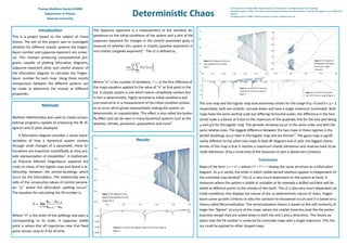
Results
Figure 1. BF diagram of the
logistic map equation for the
range 0<μ<4.
Figure 2. BF diagram of the sine
map equation for the range
0<μ<1.
Conclusion
Maps of the form where display the same structure on a bifurcation
diagram. As μ is varied, the order in which stable period solutions appear is independent of
the unimodal map iterated2
.The LE is very much dependant on the system at hand, it
measures where the system is stable or unstable so for example a duffed oscillator will be
stable at different points to the climate of the Earth. The LE is also very much dependant on
initial conditions, this displays the nature of the un-deterministic nature of chaos. Feigen-
baum came up with a theory on why the constant he discovered occurs and it is based on a
theory called Renormalization. The renormalization theory is based on the self-similarity of
larger the “figtree” structure of the maps where the smaller branches look like the earlier
branches except they are scaled down in both the and x and μ directions. This theory ex-
plains how the FB number is universal for unimodal maps with a single maximum. This the-
ory could be applied to other shaped maps.Figure 3. LE plot of the logistic map for the same range as
figure 1.
Figure 2. LE plot of the sine map
equation for the same range as
figure 2.
Figure 2. BF diagram of
the gaussian map equa-
tion for the range –
0.5<μ<0.5.
The sine map and the logistic map look extremely similar for the range 0<μ <3 and 0 < μ < 1
respectively, both are smooth, concave down and have a single maximum (unimodal). Both
maps have the same vertical scale but differing horizontal scales, the difference in the hori-
zontal scale is a factor of 4 due to the maximum of the quadratic line for the sine plot being
μ and μ/4 for the logistic map. The periodic windows occur in the same order and with the
same relative sizes. The biggest difference between the two maps in these regimes is the
period doublings occur later in the logistic map and are thinner3
. The gauss map is signifi-
cantly different to the other two maps in both BF diagram and LE plot, the biggest charac-
teristic of this map is that it reaches a maximum chaotic behaviour and reverses back to pe-
riodic behaviour. Only a small area of the Gaussian LE plot is above zero (chaotic).
Figure 6. LE plot of the Gaussian
map for the same range as figure 5.
.
.