How analytics reporting can identify and solve paratransit service shortcomings.

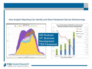
1. How Analytic Reporting Can Identify and Solve Paratransit Service Shortcomings
Will Rodman
VP, Business
Development
TSS Paratransit

2. Let’s Start at the Start
A goal of most paratransit systems: to minimize
unit costs while maintaining service standards.
What is the “right” balance of
Cost Efficiency (CE) and Service Quality (SQ)
for your system.
2
SQ
SQ
SQ CE
CE
CE

3. 3
Achieving the Optimal Balance btw
Cost Efficiency and Service Quality
 Cost efficiency measured in cost per trip
 Cost efficiency mostly derived from:
 Competitive service provider rates and incentives
 Productive schedules; reducing miles thru shared-rides
 Run structures that mirror demand profile
 Strategic use of non-dedicated service providers
SQ
CE
A truism: The tighter
the schedule, the
more OTP is reduced.

4. 4
Achieving the Optimal Balance btw
Cost Efficiency and Service Quality
 Cost efficiency measured in cost per trip
 Cost efficiency mostly derived from:
 Competitive service provider rates and incentives
 Productive schedules; reducing miles thru shared-rides
 Run structures that mirror demand profile
 Strategic use of non-dedicated service providers
SQ
CE
A truism: The tighter
the schedule, the
more OTP is reduced.

5. What is a Run Structure?
5
5 6 7 8 9 10 11 12 1 2 3 4 5 6 Serv Hrs Pay Hours
1 1 1 1 1 1 1 1 1 8 9
2 1 1 1 1 1 1 1 1 8 9
3 1 1 1 1 1 1 1 7 9
4 1 1 1 1 1 1 1 7 9
5 1 1 1 1 1 1 1 7 9
6 1 1 1 1 1 1 1 7 9
7 1 1 1 1 1 1 1 7 9
8 1 1 1 1 1 1 1 7 9
0 2 2 8 8 6 3 3 6 8 8 2 2 0 58 72
8
7
6
5
4
3
2
1
5 6 7 8 9 10 11 12 1 2 3 4 5 6

6. What is a Demand Profile?
6
 Graph of trips per
hour for each hour or
half hour of the
service day
 Superimpose demand
profile on run
structure based on
current productivity

7. Run Structure vs. Demand Profile
7
Tuesday (10-5-04) - Ridership and Capacity
0
5
10
15
20
25
30
4 5 6 7 8 9 10 11 12 1 2 3 4 5 6 7 8 9 10 11 12+
Time of Day
Runs
0
10
20
30
40
50
60
Trips
Template Runs
Actual Runs
Ridership

8. Case Study #1
8
Addressing a Suboptimal Run Structure

9. Case Study #1: The Problem
9
 OTP really low overall
 OTP really low in afternoon (54-82%)
 Not enough supply of service in the afternoon
 Could existing run start times be shifted to increase
supply of service in the afternoon?

10. Case Study #1: The Guidelines
10
 Short-term band aids needed until runs re-bid
 Increase the capacity between the hours of 13:00
and 19:00, when OTP is the lowest.
 Minimize number of runs impacted
 Focus: shift runs from oversupply periods
 Cost neutral solutions
 Band Aid #1: Shift runs w/o adjusting run length
 Band Aid #2: Shift runs with length adjustments

11. Before OTP – Week of 6/12/17
Trip Type On-Time Percentage
ADA Paratransit Trips 84.94%
Premium Trips 86.69%
11
OTP in Afternoon = 54% to 82%

12. BA #1: Shift Run Start Times Only
12
 What do we
notice?
 Over-supply
 <9:00 am
 >3:00 pm
 Under-supply
 9:00-noon
 1:00-3:00
 BA #1 solution (blue) - addresses problem time

13. BA #2: Start Times & Adjustments
13
 Extended some
AM shifts from 8
to 10 hours
 More capacity
added from
noon to 6 pm
 OTP problem in
afternoon
addressed

14. Before and After OTP
Trip Type OTP
Week of
6/12/17
OTP
Week of
11/6/17
ADA Para Trips 84.94% 90.86%
Premium Trips 86.69% 94.99%
14

15. Before and After Productivity
Trips - Week
of 6/12/17
Trips - Week
of 9/25/17
Before
Productivity
After
Productivity
Monday 2053 2082 (1.4%) 1.434 1.504 (4.9%)
Tuesday 2329 2351 (0.9%) 1.485 1.539 (3.6%)
Wednesday 2384 2455 (3.0%) 1.479 1.537 (3.9%)
Thursday 2429 2435 (0.2%) 1.497 1.567 (4.7%)
Friday 2075 1975 (-4.8%) 1.456 1.534 (5.4%)
15
Productivity increases = 3.6% to 5.4%

16. Before and After and After OTP
Trip Type OTP
Week of
6/12/17
OTP
Week of
11/6/17
OTP
Week of
2/5/18
ADA Para Trips 84.94% 90.86% 94.72%
Premium Trips 86.69% 94.99% 95.17%
16

17. Optimization Tools
 Temporal/geographic analysis of
accommodated demand, unassigned
trips
 Filters to perform analyses of providers,
fleets, vehicle types, service areas,
days/times, dedicated vs. non-dedicated
service providers
 Detail and summary (various
subgrouping) of scheduling results
 Individual itinerary assessment 17

18. Optimization Tools (continued)
 Provides the ability to:
 Modify run structure and forecast results
 Assess impact of seasonal parameters
 Assess impact of changing scheduling or on-
time windows, provider cost, veh. capacity,
changes in service zones, transfer points
 As input, any previously recorded
scheduling snapshot can be loaded in
and analyzed
18

19. Impacts on Key Metrics
 Provides the ability to:
 Modify run structure and forecast results
 Assess impact of seasonal parameters
 Assess impact of changing scheduling or on-
time windows, provider cost, vehicle
capacity, changes in service zones, transfer
points, etc.
 As input, any previously recorded
scheduling snapshot loaded / analyzed
19

20. Metrics and More Metrics
 Number of Vehicles (Resources)
Available, Used (Needed) and Utilization
 Number of Revenue Vehicle Hours
 Driver Regular Hours – Available, Used
 Driver Overtime Hours – Available, Used
 Idle Time, Dwell Time, Deadhead Time
 Average Productivity – Trips per RVH,
Direct Miles per RVH
20

21. Metrics and More Metrics (cont’d)
 Percentage of Shared Trips
 Average Distance – Total and Direct
 Average Travel Time – Total and Direct
 Average Speed – Total and Direct
 Trips Assigned – Total, amb, w/c
 Trips Unassigned – Total, amb, w/c
 Percentage of On-Time and Late Trips
 Cost per trip, cost per RVM
21

22. Active & Inactive Service Supply
22

23. Unassigned Trips
23

24. Strategies / Simulations
 1 Adjusted Start Times; Run Lengths Unchanged
 2 Eliminated Zones and Inter-Zone Transfers
 3 Scenarios 1+ 2
 4 Scenario 3 plus 15% cancellations
 5 Scenario 4; 10% advance + 5 % late/no-shows
 6 Scenario 5 plus NDSPs
24

25. The Results
Scenario Vehicles Productivity Cost Per Trip Unassigned
Base 645 1.47 $33.96 358
1 645 1.49 $31.61 152
2 645 1.49 $33.63 326
3 645 1.49 $33.46 6
4 603 1.32 $37.91 --
5 572 1.42 $35.17 36
6 653/33 1.43 $34.69 --
25
Scheduling Tests Scheduling Tests and Simulations
1 Adjusted Start Times 4 Scenario 3 plus 15% cancellations
2 Eliminated Zones/Transfers 5 Scenario 4; 10% adv + 5 %lates/NS
3 Scenarios 1+ 2 6 Scenario 5 plus NDSPs

26. Case Study #2
26
Addressing a Suboptimal Service Mix

27. Case Study #2:
Run Structure vs. Demand Profile - October 2004
27
Tuesday (10-5-04) - Ridership and Capacity
0
5
10
15
20
25
30
4 5 6 7 8 9 10 11 12 1 2 3 4 5 6 7 8 9 10 11 12+
Time of Day
Runs
0
10
20
30
40
50
60
Trips
Template Runs
Actual Runs
Ridership

28. 28
0
5
10
15
20
25
30
35
40
45
50
Monday Vehicles in Service vs. Vehicles Required by Time Period
Vehicles in Service
Vehicles Required
Active Vehicles
0
5
10
15
20
25
30
35
40
45
50
Tuesday Vehicles in Service vs. Vehicles Required by Time Period
Vehicles in Service
Vehicles Required
Active Vehicles
0
5
10
15
20
25
30
35
40
45
50
Wednesday Vehicles in Service vs. Vehicles Required by Time Period
Vehicles in Service
Vehicles Required
Active Vehicles
0
5
10
15
20
25
30
35
40
45
50
Thursday Vehicles in Service vs. Vehicles Required by Time Period
Vehicles in Service
Vehicles Required
Active Vehicles
0
5
10
15
20
25
30
35
40
Friday Vehicles in Service vs. Vehicles Required by Time Period
Vehicles in Service
Vehicles Required
Active Vehicles
Case Study #2:
Run Structure vs. Demand Profile – May 2012

29. Case Study #2:
Run Structure Optimization Test – May 2012
29
Weekly
Total
Vehicle
Hours
Weekly
Driver
Hours
Max
Vehicles
in Service
Existing 2704 2887 52
Optimized 2674 2850 51
Difference -1.1% -1.3% -1.9%

30. Case Study #2:
Service Mix Analysis - May 2012
30
 Diverting peak period
trips had diminishing
returns. Why?
 Because weekday
dedicated run structures
were close to optimal
 Diverting trips to NDSPs
during low-demand
times (evenings and
weekends) produced the
most savings

31. Thank you!
Questions?
31