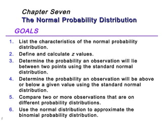
1. l
Chapter Seven
The Normal Probability DDiissttrriibbuuttiioonn
GOALS
1. List the characteristics of the normal probability
distribution.
2. Define and calculate z values.
3. Determine the probability an observation will lie
between two points using the standard normal
distribution.
4. Determine the probability an observation will be above
or below a given value using the standard normal
distribution.
5. Compare two or more observations that are on
different probability distributions.
6. Use the normal distribution to approximate the
binomial probability distribution.

2. Distribusi Probabilitas KKoonnttiinnyyuu
 Distribusi probabilitas kontinyu: didasarkan
pada variabel acak kontinyu biasanya
diperoleh dengan mengukur.
 Dua bentuk distribusi probabilitas kontinyu:
Distribusi probabilitas seragam (uniform)
Distribusi probabilitas normal

3. Normal Distribution
Importance of Normal Distribution
1. Describes many random processes or
continuous phenomena
2. Basis for Statistical Inference

4. Characteristics of a Normal
Probability Distribution
 The normal curve is bell-shaped and has a single peak at
the exact center of the distribution.
 The arithmetic mean, median, and mode of the
distribution are equal and located at the peak . Thus half
the area under the curve is above the mean and half is
below it.
 The normal probability distribution is unimodal=only one
mode.
 It is completely described by Mean & Standard Deviation
 The normal probability distribution is asymptotic. That is
the curve gets closer and closer to the X -axis but never
actually touches it.

5. Normal Probability distribution
2
2
é ù -ê x
- ú
m
s
( )
Normal Probability
distribution
( ) 1 2
= êë úû
P x e
s p
2
e=2.71828
Do not worry about the formula, you do not need to
calculate using the above formula.

6. The density functions of normal distributions with
zero mean value and different standard deviations
Bell-shaped
Symmetric
Mean=median = mode
Unimodal
Asymptotic

7. Difference Between Normal Distributions
x
x
x
(a)
(b)
(c)

8. Normal Distribution Probability
Probability is the area
under the curve!
f(X) A table may be
constructed to help
us find the probability
c d X

9. Infinite Number of Normal Distribution Tables
Normal distributions differ by
mean & standard deviation.
Each distribution would
require its own table.
X
f(X)

10. Distribusi Probabilitas Normal Standar
 Distribusi Normal Standar adalah distribution
normal dengan mean= 0 dan standar
deviasi=1.
 Juga disebut z distribution.
 A z- value is the distance between a selected
value, designated X , and the population mean
m, divided by the population standard
deviation, s. The formula is:
z =X -m
s

11. The Standard Normal Probability
Distribution
 Any normal random variable can be
transformed to a standard normal random
variable
 Suppose X ~ N(μ, s 2)
Z=(X-μ)/ s ~ N(0,1)
P(X<k) = P [(X-μ)/ s < (k-μ)/ s ]

12. Standardize the Normal Distribution
Standardized Normal
Distribution
m Z = 0
s z = 1
Z
Normal
Distribution
Z = X -m
m X
s
s
Because we can transform any normal random variable into
standard normal random variable, we need only one table!

13. Transform to Standard Normal Distribution
A numerical example
 Any normal random variable can be transformed to a
standard normal random variable
x x-m (x-m)/σ x/σ
0 -2 -1.4142 0
1 -1 -0.7071 0.7071
2 0 0 1.4142
3 1 0.7071 2.1213
4 2 1.4142 2.8284
Mea
n
2 0 0 1.4142
std 1.4142 1.4142 1 1

14. Standardizing Example
Data of weight of children under 5 years old in Kg. Mean
(m)= 5 and s= 10. What is the probability of children
weighted at 5 Kgs to 6.2 Kgs?
s Z = 1
m = 0
.12
Z Z Normal
Distribution
Standardized Normal
Distribution
= - =6.2-5=
s
m = 5 X
s = 10
6.2
0.12
10
Z X m

15. Obtaining the Probability
s Z = 1
m = 0
0.12
Z Z Standardized Normal
Probability Table (Portion)
Z .00 .01
0.0 .0000 .0040 .0080
.0398 .0438
0.2 .0793 .0832 .0871
0.3 .1179 .1217 .1255
0.0478
.02
0.1 .0478
Probabilities
Shaded Area
Exaggerated

16. Example P(3.8 £ X £ 5)
Standardized Normal
Distribution
s Z = 1
m Z = 0 Z
-0.12
Normal
Distribution
0.0478
= - =3.8-5=-
s
m = 5 X
Shaded Area Exaggerated
s = 10
3.8
0.12
10
Z X m

17. Example (2.9 £ X £ 7.1)
Standardized Normal
0
Distribution
s Z = 1
-.21 .21 Z
Normal
Distribution
.1664
.0832 .0832
X
X
-
Shaded Area Exaggerated
5
s = 10
Z
Z
=
2.9 7.1 X
=
-
= -
=
-
=
-
=
m
s
m
s
2 .
9 5
.
21
10 7 .
1 5
.
21
10

18. Example (2.9 £ X £ 7.1)
Standardized Normal
0
Distribution
s Z = 1
-.21 .21 Z
Normal
Distribution
.1664
.0832 .0832
X
X
-
Shaded Area Exaggerated
5
s = 10
Z
Z
=
2.9 7.1 X
=
-
= -
=
-
=
-
=
m
s
m
s
2 .
9 5
.
21
10 7 .
1 5
.
21
10

19. Example P(X ³ 8)
s Z = 1
.5000 .3821
m Z = 0
.30
Z Normal
Distribution
Standardized Normal
Distribution
.1179
Shaded Area Exaggerated
Z
X
=
-
=
-
=
m
s
8 5
10
.30
s = 10
m = 5 8
X

20. Example P (7.1 £ X £ 8)
Standardized Normal
m z = 0
Distribution
s Z = 1
.1179 .0347
.21 .30 Z
Normal
Distribution
.0832
Z X
Shaded Area Exaggerated
Z
X
=
-
=
-
=
=
-
=
-
=
m
s
m
s
71 .
5
.
21
10 8 5
.
30
10
s = 10
m = 5
7.1 8 X

21. Normal Distribution Thinking Challenge
 You work in Quality Control for GE. Light
bulb life has a normal distribution with μ=
2000 hours & s = 200 hours. What’s the
probability that a bulb will last
between 2000 & 2400 hours?
less than 1470 hours?

22. Solution P (2000 £ X £ 2400)
Standardized Normal
Distribution
s Z = 1
m Z Z = 0
2.0
Normal
Distribution
.4772
Z
X
=
-
=
-
=
m
s
2400 2000
200
2.0
s = 200
m = 2000 2400
X

23. Solution P (X £ 1470)
Standardized Normal
Distribution
s Z = 1
.5000
m Z= 0 Z
-2.65
Normal
Distribution
.0040 .4960
Z
X
=
-
=
-
= -
m
s
1470 2000
200
2.65
m = 2000 X
s = 200
1470

24. Finding Z Values for Known
Probabilities
Standardized Normal
Probability Table (Portion)
.1217 .01
Z .00 .02
0.0 .0000 .0040 .0080
0.1 .0398 .0438 .0478
0.2 .0793 .0832 .0871
.1179 .1255
s Z = 1
m Z = 0 .31
Z
0.3 .1217
What Is Z Given
P(Z) = 0.1217?
Shaded Area
Exaggerated

25. Finding X Values for Known
Probabilities
Normal Distribution Standardized Normal Distribution
s Z = 1
m = 5 X .31
m Z = 0 Z
s = 10
?
.1217 .1217
X =m +Z×s =5+(0.31)×10=8.1
Shaded Area Exaggerated

26. EXAMPLE 1
 The bi-monthly starting salaries of recent MBA
graduates follows the normal distribution with
a mean of $2,000 and a standard deviation of
$200. What is the z- value for a salary of
$2,200?
z = X -
m
$2,200 $2,000 1.00
$200
s
= - =

27. EXAMPLE 1 continued
 What is the z-value of $1,700 ?
z = X -
m
s
=$1,700 -$2,200 =-
1.50
$200
 A z-v alue of 1 indicates that the value of
$2,200 is one standard deviation above
the mean of $2,000.
 A z-v alue of –1.50 indicates that $1,700 is
1.5 standard deviation below the mean of
$2000.

28. Areas Under the Normal Curve
 About 68 percent of the area under the normal
curve is within one standard deviation of the
mean. m ± s
P(m - s < X < m + s) = 0.6826
 About 95 percent is within two standard
deviations of the mean. m ± 2 s
P(m - 2 s < X < m + 2 s) = 0.9544
 Practically all is within three standard
deviations of the mean. m ± 3 s
P(m - 3 s < X < m + 3 s) = 0.9974

29. Areas Under the Normal Curve
Between:
± 1 s - 68.26%
± 2 s - 95.44%
± 3 s - 99.74%
μ
μ-2σ μ+2σ
μ-3σ μ-1σ μ+1σ
μ+3σ

30. EXAMPLE 2
 The daily water usage per person in
Surabaya is normally distributed with a
mean of 20 gallons and a standard
deviation of 5 gallons. About 68
percent of those living in Surabaya will
use how many gallons of water?
 About 68% of the daily water usage will
lie between 15 and 25 gallons.

31. EXAMPLE 3
 What is the probability that a person from
Surabaya selected at random will use
between 20 and 24 gallons per day?
= - =20-20 =
0.00
5
z X m
s
= - =24-20 =
0.80
5
z X m
s
P(20<X<24)
=P[(20-20)/5 < (X-20)/5 < (24-20)/5 ]
=P[ 0<Z<0.8 ]

32. The Normal Approximation to the
Binomial
 The normal distribution (a continuous
distribution) yields a good approximation of
the binomial distribution (a discrete
distribution) for large values of n.
 The normal probability distribution is
generally a good approximation to the
binomial probability distribution when n p
and n(1- p ) are both greater than 5.

33. The Normal Approximation continued
Recall for the binomial experiment:
 There are only two mutually exclusive
outcomes (success or failure) on each
trial.
 A binomial distribution results from
counting the number of successes.
 Each trial is independent.
 The probability is fixed from trial to trial,
and the number of trials n is also fixed.

34. The Normal Approximation
normal
binomial

35. Continuity Correction Factor
 The value 0.5 subtracted or added, depending on
the problem, to a selected value when a binomial
probability distribution (a discrete probability
distribution) is being approximated by a continuous
probability distribution (the normal distribution).
Four cases may arise:
 For the P at least X occur, use the area above (X – 0,5)
 For the P that more than X occur, use the area above (X +
0,5)
 For the P that X or fewer occur, use the area below (X +
0,5)
 For the P that fewer than X occur, use the area below (X –
0,5)

36. Continuity Correction Factor
 Because the normal distribution can take all real
numbers (is continuous) but the binomial distribution
can only take integer values (is discrete), a normal
approximation to the binomial should identify the
binomial event "8" with the normal interval "(7.5, 8.5)"
(and similarly for other integer values). The figure
below shows that for P(X > 7) we want the magenta
region which starts at 7.5.

37.  n=20 and p=0.25 P(X ≥ 8)=?
 First step: determine mean (m) & standard deviation (s)
m = np = (20)(0.25) = 5
s = np (1-p ) = (5)(1-0.25) = 3.57 =1.94
 Second step: determine the z-value
 Third step: check the area below normal curve

38. 1. Without correction factor of 0.5:
= - = - =
8 5 1.55
1.94
z X m
s
check in table-Z: P(X ≥ 8)=0.5-0.4394=0.0606
2. With correction factor of 0.5: P(X ≥ 8) P(X ≥ 8-0.5=7.5)
= - = - =
7.5 5 1.29
1.94
z X m
s
check in table-Z: P(X ≥ 7.5)=0.5-0.4015=0.0985
 The exact solution from binomial distribution function is
0.1019.
 The continuity correct factor is important for the
accuracy of the normal approximation of binomial.
 The approximation is quite good.

39. EXAMPLE 5
A recent study by a marketing research firm showed
that 15% of American households owned a video
camera. For a sample of 200 homes, how many of the
homes would you expect to have video cameras?
 What is the mean?
m =np =(.15)(200) =30
 What is the variance?
s 2 = np(1-p ) =(30)(1-.15) = 25.5
 What is the standard deviation?
s= 25.5 =5.0498

40. EXAMPLE 5 continued
What is the probability that less than 40
homes in the sample have video cameras?
 We use the correction factor, so X is 39.5.
 The value of z is 1.88.
1.88
= - = 39.5 -30.0 =
5.0498
z X m
s

41. Example 5 continued
 From Appendix D the area between 0 and 1.88
on the z scale is .4699.
 So the area to the left of 1.88 is
.5000 + .4699 = .9699.
 The likelihood that less than 40 of the 200
homes have a video camera is about 97%.

42. EXAMPLE 5
P(z< 1.88)
=.5000+.4699
=.9699
z =1.88
0 1 2 3 4
z

43. Soal
 KPS MP melakukan polling dengan
menyebarkan 60 kuisioner. Probabilitas
kembalinya kuisioner adalah 80%. Hitung
probabilitas :
50 kuisioner kembali
Antara 45-55 kuisioner kembali
Kurang dari 55 kuisioner kembali
20 atau lebih kuisioner kembali

44. Chapter Seven
The Normal Probability DDiissttrriibbuuttiioonn
- END -