Excel notes by satish kumar avunoori
•
2 gefällt mir•829 views

Excel notes for beginners notes developed based on the osmania university

Empfohlen
Weitere ähnliche Inhalte
Was ist angesagt?
Was ist angesagt? (20)
Ähnlich wie Excel notes by satish kumar avunoori
Ähnlich wie Excel notes by satish kumar avunoori (20)
Kürzlich hochgeladen
Kürzlich hochgeladen (20)
Excel notes by satish kumar avunoori
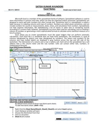
- 1. SATISH KUMAR AVUNOORI Excel Notes Unit – I INTRODUCTION TO MS – EXCEL Microsoft Excel is a member of the spreadsheet family of software. Spreadsheet software is used to store information in columns and rows, which can then be organized and/or processed. Spreadsheets are designed to work well with numbers but often include text. Sometimes text in a spreadsheet is called a label, because it is labeling columns and rows of numbers. Numbers are called values sometimes, and can include numbers for counts or measurements, dates, times, and calculations from numbers. Spreadsheets can help organize information, like alphabetizing a list of names or other text or reordering records according to a numeric field. However, spreadsheets are more often used for calculating, such as totaling a column of numbers or generating a more sophisticated formula to calculate some statistical measure on a list of numbers. Excel allows you to create spreadsheets much like paper ledgers that can perform automatic calculations. Each Excel file is a workbook that can hold many worksheets. The worksheet is a grid of columns (designated by letters) and rows (designated by numbers). The letters and numbers of the columns and rows (called labels) are displayed in gray buttons across the top and left side of the worksheet. The intersection of a column and a row is called a cell. Each cell on the spreadsheet has a cell address that is the column letter and the row number. Cells can contain either text, numbers, or mathematical formulas. Excel 2010 Screen Elements: CREATING AND EDITING WORKSHEET: CREATING A NEW WORKSHEET: By default excel consist of three new blank work sheets To add new works sheet: (Shift + F11) Steps: Right Click the Sheet Name(Sheet1, Sheet2, Sheet3) and select Insert option. Insert dialogue window will open Choose the Worksheet from that Click on ok button Sheet 4 will created BA-II Yr- SEM IV Simple way to learn excel
- 2. Page 2 of 8 HOW TO RENAME THE SHEET LABEL: By default sheet names were (Sheet1, Sheet2….), to change the Sheet1 to for example ( TICSA ) Steps: Right Click on the Sheet Name (Sheet1) and select Rename option. Now type the sheet name to TICSA HOW TO DELETE THE SHEET Steps: Right Click on the Sheet Name Ex: Sheet2 Choose the option Delete Now Sheet3 will be deleted HOW TO HIDE THE SHEET Steps: Right Click on the Sheet Name (Ex: Sheet2) fromSheet1, Sheet2 and Sheet3 Choose the option Hide Now Sheet2 will be Hide HOW TO UN HIDE THE SHEET Steps: Right Click on the Sheet Name (Ex: Sheet1 or 3) from Sheet1, Sheet3 Choose the option Unhide Unhide window will open In that window we can see the list of sheets which were hidden From that list select the sheet you need (Ex: Sheet2) Now Sheet2 will be un-hidden successfully Short Cuts: To move from Sheet1 to Sheet2 (Ctrl + Page Down) key To move from Sheet2 to Sheet1 (Ctrl + Page Up) key To move the cursor up/down one by one (Up arrow / Down arrow) To move the cursor right / le one by one (Right arrow / Le arow) To move the cursor towards the down / up in certain amounts(Page Down / Page Up) Key To move the curosr towards right/Le in certain amounts (Alt Page Up / Alt Page Down) Keys To Edit the data in the cells (Function key : F2) FORMAT CELLS: One of the most powerful tools in Excel is the ability to apply specific formatting for text and numbers. Instead of displaying all cell content in exactly the same way, you can use formatting to change the appearance of dates, times, decimals, percentages (%), currency ($), and much more. Steps: Select Ex: Column B Right click choose option format cellsFormatCellswindow will open from that select Number tab Choose option Currency from the option symbol list Select option Rs Urdu Now Column B Amount changes with Rs symbol Note: Same Procedure for to change Number, Date, Time, Currency, Percentage etc. MERGE CELLS: Merging cells is often used when a title is to be centred over a particular section of a spreadsheet. When a group of cells is merged, only the text in the upper-leftmost box is preserved. Steps:Highlight or select a range of cells. Right-click on the highlighted cells and select Format Cells... Click the Alignment tab and place a checkmark in the checkbox labelled Merge cells. Before Merge After Merge Note : Follow same steps for to do Wrap text and shrink to fit
- 3. Page 3 of 8 ARITHMETIC OPERATIONS (Addition +, Subtraction -, Multiplication *, Division /, …)
- 4. Page 4 of 8 FUNCTIONS: =Min() : find the smallest number in a range of cells =Max():find the largest number contained in a range of cells =Trim(): Remove excess whitespace =Len():It will show how many characters are in cell =Concatenate():Two cells and turns it into one =Round():This function lets you round off numbers. ROUND requires two arguments: a number or cell, and the number of digits to round to. =Sqrt(): Returns the square root of a number =Power() : returns the result of number raised to a power =left() : returns specified no. of characters from the start of a text string =Right(): returns specified no. of characters form the end of a text string
- 5. Page 5 of 8 COMPARISON OPERATORS:(Equal =, Greater than >, Greaterthan or Equal to >=, Less than <, Less than or equal to <=, Not equal<> IF STATEMENTS: SIMPLE IF: Check whether given condition is met, Returns one value if true, andanother value if false. Syntax : IF( condition, [value_if_true], [value_if_false] ) NESTED IF: Nest multiple IF functions within one Excel formula. Simply we can say if within the if. Syntax: if ( condition1, value_if_true1, IF( condition2, value_if_true2, value_if_false2 )) LOGICAL FUNCTIONS: AND, OR, NOT AND: Returns TRUE if all of the arguments evaluate to TRUE. OR: Returns TRUE if any argument evaluates to TRUE. From the above table any of the condition should be satisfied.
- 6. Page 6 of 8 NOT: Returns the reversed logical value of its argument. I.e. If the argument is FALSE, then TRUE is returned and vice versa. STATISTICAL FUNCTIONS: (Mean, Median, Mode) CHART A chart is a graphical representation of data, in which "the data is represented by symbols, such as bars in a bar chart, lines in a line chart, or slices in a pie chart". A chart can represent tabular numeric data, functions or some kinds of qualitative structure and provides different info Example : Bar Chart PIVOT TABLE A pivot table is a table that summarizes data in another table, and is made by applying an operation such as sorting, averaging, or summing to data in the first table, typically including grouping of the data. Steps: Keeps Source in sheet1 as shown in below Select Insert Tab Choose the option Pivot Table Pivot Table Create Pivot table window will open Select the radio button table or range Select total source Click on ok button Now Pivot table will be appear in sheet4 Sheet1 Sheet4
- 7. PIVOT CHART: Steps: Keeps Source in sheet1 as shown in below Select Insert Tab Choose the option Pivot Table Pivot Chart Create Pivot table with Pivot chart window will openSelect the radio button table or range Select total source Click on ok button Now Pivot Chart will be appear in sheet4 Same Source of example which is used for to create Pivot Table CONSOLIDATE: Microsoft Excel has a data consolidation feature that allows multiple tables to be consolidated into a single summary report. Consolidating the data often enables easier editing and viewing of information since it can be seen in aggregate form as a master spreadsheet. There are three basic ways to consolidate data in Excel: by position, category and formula. To locate the command, start by selecting the Data menu and then the Consolidate command, which will then prompt you to select one of the three consolidation options. Steps for Linking and Consolidation: Sheet1 as shown below Sheet2 as shown below Sheet3 as shown below Sheet4 as shown below Steps: In Sheet1, Sheet2, Sheet3 in cell address Total (F3) Write the formula =SUM(C3:D3) Click and drag up to F6 address Steps to do CONSOLIDATE: Now Click on cell C3 Under the DATA tab, in the Data Tools group, click on Consolidate. It will display the following Dialog Box
- 8. The worksheet Consolidate Look Like below LINKING worksheets, click on the Sheet5 Click on Data tab and then click on Consolidate under the Data Tools group. The consolidate dialog box will appear. Repeat step a) to e) which at side of the consolidate dialogue box in the above. • Click on the check box “Create links to source data” • Click OK. There is no difference between Linking and Consolidation except that if you change the data in the source pages, it will not make any change in the Consolidation worksheet, whereas any modification on the data of the source worksheets will automatically update the data on the Link worksheet. Steps: a) Click on the ‘Reference’ text box. b) Click on Sheet1 and select cells B3 to D7 and click on the Add button. c) Click on Sheet2 and click on Add button. d) Click on Sheet3 and click on Add button. e) Click OK The worksheet consolidate should now report the sum of Marks of all the students of I Yr, II Yr and III Yr for each subject. FOR ONLINE CLASSES CONTACT skype: avunoori123 satishkumar.avunoori@gmail.com