Recent developments in the field of reduced order modeling - and in particular, active subspace construction - have made it possible to efficiently approximate complex models by constructing low-order response surfaces based upon a small subspace of the original high dimensional parameter space. These methods rely upon the fact that the response tends to vary more prominently in a few dominant directions defined by linear combinations of the original inputs, allowing for a rotation of the coordinate axis and a consequent transformation of the parameters. In this talk, we discuss a gradient free active subspace algorithm that is feasible for high dimensional parameter spaces where finite-difference techniques are impractical. We illustrate an initialized gradient-free active subspace algorithm for a neutronics example implemented with SCALE6.1.

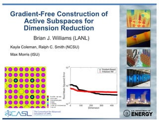
1. Kayla Coleman, Ralph C. Smith (NCSU)
Max Morris (ISU)
Gradient-Free Construction of
Active Subspaces for
Dimension Reduction
Brian J. Williams (LANL)
Dimension
0 100 200 300 400
RootMeanSquaredError
10
-4
10
-3
10-2
Gradient-Based
Initialized AM
!
6 ss-304 - bpr clad
5 air in bprs
4 borosilicate glass
3 water
2 cladding
1 2.561 wt % enriched fuel
7 rod n-9
6 ss-304 - bpr clad
5 air in bprs
4 borosilicate glass
3 water
2 cladding
1 2.561 wt % enriched fuel
7 rod n-9

2. 2
Abstract
Recent developments in the field of reduced order modeling - and in
particular, active subspace construction - have made it possible to
efficiently approximate complex models by constructing low-order
response surfaces based upon a small subspace of the original high
dimensional parameter space. These methods rely upon the fact that
the response tends to vary more prominently in a few dominant
directions defined by linear combinations of the original inputs,
allowing for a rotation of the coordinate axis and a consequent
transformation of the parameters. In this talk, we discuss a gradient
free active subspace algorithm that is feasible for high dimensional
parameter spaces where finite-difference techniques are impractical.
We illustrate an initialized gradient-free active subspace algorithm for
a neutronics example implemented with SCALE6.1, for input
dimensions up to 7700.

3. 3
Dimension Reduction
• The statistics community has been interested in dimension reduction
methods for regression problems for 25+ years
– Introduction of sliced inverse regression (SIR) and sliced average
variance estimation (SAVE) in 1991
• Statistical formulation: Estimate the central subspace
– Regress response Y = f(X) on a random m-vector of inputs X
– Intersection of all subspaces ! with the property that Y is conditionally
independent of X given the projection of X onto !
– Result is a set of n < m orthogonal linear combinations of X
• [Xia, Annals of Statistics 2007] introduced nonparametric methods to
estimate ! exhaustively
– Compared performance to SIR, SAVE, principal Hessian direction (PHD),
and minimum average variance estimation (MAVE)
• [Cook et al., JASA 2009] introduced a likelihood method for
estimating ! termed likelihood acquired directions (LAD)
– Compared performance to SIR, SAVE, and directional regression (DR)
– Assumes conditional normality but robust to non-normality
– Likelihood ratio statistic, AIC, BIC used to choose n

4. 4
Active Subspaces
Motivation:
• Some UQ problems involve high-dimensional input spaces that present
challenges for standard surrogate and model calibration algorithms
– e.g. 7700 cross section perturbations in a PWR quarter fuel lattice
– 10k – 100k+ parameters possible in CIPS Challenge Problem
• Typically sensitivity analysis would substantially reduce this dimension as
most parameters have a relatively small influence on the QoIs
• Popular active subspace methods seek to find a substantially reduced set
of parameters formed as linear combinations of the original parameters
– Conceptual similarities to statistical dimension reduction methods
– If possible identify a set of 100 or fewer active parameters
• Use gradients to identify active parameters if they are produced by the
code. Otherwise, gradient free approaches must be considered
– Active area of research
Goal: Using a new gradient free algorithm for active subspace
discovery, determine active parameters for use in surrogate
construction and model calibration

5. 5
Active Subspace Construction
Example:
• Varies most in [0.7, 0.3] direction
• No variation in orthogonal direction
y = exp(0.7x1 + 0.3x2)
!
Strategy:
• Employ gradient-based or gradient-free techniques, in combination with
SVD or QR to construct active subspace.
• Employ active subspaces for:
- Linear Karhunen-Loeve expansion-based UQ
- Surrogate or reduced-order model construction
- Model calibration
• Outputs may vary significantly in only a
few “active” directions, which may be
linear combinations of inputs.
Note:

6. 6
Gradient-Based Active Subspace
Active Subspace: See [Constantine, SIAM 2015]. Consider
f = f(x), x 2 X ✓ Rm
and
rxf(x) =

@f
@x1
· · ·
@f
@xm
T
Construct outer product
Partition eigenvalues:
Rotated Coordinates:
C = W⇤WT
⇤ =

⇤1
⇤2
, W = [W1 W2]
y = WT
1 x 2 Rn
and z = WT
2 x 2 Rm n
C =
Z
(rxf)(rxf)T
⇢dx
r(x) : distribution of input x parameters

7. 7
Motivation
Results:
(1) i =
Z ⇣
(rxf)
T
wi
⌘2
⇢(x) dx
Derivative of f(x) in the direction wi
Z
(rzf)
T
(rzf) ⇢(x) dx = n+1 + · · · + m(2)
• n can be chosen by looking for a ”large” gap between ln and ln+1,
such that ln+1 + … + lm is relatively “small”
f(x) ⇡ g(WT
1 x)(3) g is a link function

8. 8
Active and Central Subspaces
• Suppose f(x) = g(y) for
• Inputs and output are therefore conditionally independent given the
active variables, and so the active subspace defined by the columns
of W1 contains the central subspace
⇡(f(x), x|y) = ⇡(g(y), x|y)
= ⇡(g(y)|y, x) ⇡(x|y)
= ⇡(g(y)|y) ⇡(x|y)
= ⇡(f(x)|y) ⇡(x|y)
y = W T
1 x

9. 9
Estimation
Approximation via Monte Carlo:
1. Draw M samples { xj } independently from r(x)
2. For each xj, compute
3. Approximate
4. Compute the eigendecomposition
rxfj = rxf(xj)
C ⇡ ˆC =
1
M
MX
j=1
(rxfj) (rxfj)
T
ˆC = ˆWˆ⇤ ˆWT
Steps 3 and 4 equivalent to computing the SVD of the gradient matrix
G =
1
p
M
[rxf1 · · · rxfM ] = ˆWˆ⇤1/2 ˆV
" = ||W1W T
1
ˆW1
ˆW T
1 ||2 = || ˆW T
1 W2||2
Error in estimated active subspace:
" 
4 1
n n+1
d is a user-specified tolerance for the
eigenvalue estimates (used to choose M)

10. 10
Order Determination
1. Gap-based
• Stop at largest gap in eigenvalue spectrum
2. Error-based
• Specify error tolerance etol, G = U L1/2 VT
a) Draw a sequence of p standard Gaussian vectors { w1, …, wp }
b) Let be the first j columns of U
c) Let
• Find smallest j for which
• Error bound holds with probability 1 – 10-p
3. PCA-based
• Stop at minimal dimension yielding variance explained in covariance matrix
formed from G exceeding user-specified threshold (e.g. 99%)
4. Response surface-based
• Use the minimal dimension required to reduce response surface error on a
validation dataset below a user-specified threshold (e.g. 0.01, 0.001)
˜Um⇥j
"j
upp = 10
p
2/⇡ max
i=1,...,p
||(I ˜U ˜UT
)G!i
||
"j
upp < "tol
Goal: Determine dimension of active subspace

11. 11
Gradient Approximation for Large Input Spaces
• Utilized when finite difference approach to gradient approximation is
computationally prohibitive; e.g., SCALE6.1 with 7700 inputs.
• Construct ellipsoid where linearity is reasonable assumption.
• Maximize function values and gradient information using “great ellipsoid”
relations.
Iteration 1
x0
x
y
z-
z+
Iteration 2
x0
x
y
z+
z-

12. 12
“Great Ellipsoid” Solution
• Consider a matrix C collecting h+1 input samples from the surface of
the unit hypersphere:
• Collect the sampled output differences into a vector y:
• The direction of steepest ascent within the column space of C is given
by:
C =
⇥
w v1 · · · vh
⇤
y =
⇥
g(w) g(0) g(v1) g(0) · · · g(vh) g(0)
⇤T
umax =
C CT
C y
q
yT (CT C) y

13. 13
SCALE6.1: High-Dimensional Example
!
6 ss-304 - bpr clad
5 air in bprs
4 borosilicate glass
3 water
2 cladding
1 2.561 wt % enriched fuel
7 rod n-9
6 ss-304 - bpr clad
5 air in bprs
4 borosilicate glass
3 water
2 cladding
1 2.561 wt % enriched fuel
7 rod n-9
PWR Quarter Fuel Lattice
materials and reactions specified in Table 3, and fix all others to their
rovided by the SCALE6.1 cross-section libraries.
ze of the input space, we use only the initialized adaptive Morris al-
ng our results to the gradient-based results obtained from the SAMS
alization algorithm allows us to begin Algorithm 2 with a subset of 147
ns rather than approximating directional derivatives in all 7700 original
The adaptive Morris algorithm is quickly able to improve upon the di-
ed by the initialization algorithm and reduce the number of important
Materials Reactions
234
92U 10
5B 31
15P ⌃t n Ñ
235
92U 11
5B 55
25Mn ⌃e n Ñ p
236
92U 14
7N 26Fe ⌃f n Ñ d
238
92U 15
7N 116
50Sn ⌃c n Ñ t
1
1H 23
11Na 120
50Sn ¯⌫ n Ñ 3
He
16
8O 27
13Al 40Zr n Ñ ↵
6C 14Si 19K n Ñ n1
n Ñ 2n
le 3: Materials and reactions for the 7700-input example.
20
Note: We cannot efficiently approximate all directional derivatives
required to approximate the gradient matrix. Requires an efficient
gradient approximation algorithm.
Setup:
• Input Dimension: 7700
• Output keff

14. 14
SCALE6.1: High-Dimensional Example
Setup:
• Input Dimension: 7700
SCALE Evaluations:
• Gradient-Based: 1000
• Initialized Adaptive Morris: 18,392
(0.20%)
• Projected Finite-Difference:
7,701,000
Active Subspace Dimensions:
Eigenvalue
0 50 100 150 200 250 300
Magnitude
10
-30
10
-20
10
-10
10
0
Gradient-Based
Initialized AM
observe the first major gaps in the eigenvalue spectrum after the first eigenvalue for both
methods. The PCA and error-based criteria yield more conservative estimates for the
gradient-based method. The error upper bounds are plotted in Figure 8(c). We observe a
steady decline in the error for the gradient-based method over the first 350 dimensions. Fo
the initialized adaptive Morris method, the errors are machine epsilon once the eigenvalue
drop o↵, since the error-based criteria is strongly related to the decay in the eigenvalue
spectrum.
The root mean squared errors (5) for the 1st-order multivariate polynomial response
surfaces are plotted in Figure 8(b) for the first 450 dimensions. The slower decay observed
n the initialized adaptive Morris errors is due to di↵erence in eigenvalue spectrum; column
3 through 450 contribute very little to the decrease in response surface error because of thei
correspondingly insignificant eigenvalues. To visually depict the accuracy of the response
surfaces, we plot the observed ke↵ values for 100 testing points versus the predicted output
using the 25-, 75-, 150-, and 300-dimensional active subspaces for the two methods in
Figure 9. As the number of dimensions increases, we observe a tighter fit to the diagona
axis that represents a perfect match in predicted versus observed outputs.
Gap PCA Error Tolerance
Method 0.75 0.90 0.95 0.99 10´3
10´4
10´5
10´6
Gradient-Based 1 2 6 9 24 1 13 90 233
Initialized AM 1 1 1 1 2 1 2 2 2
Table 4: Active subspace dimension selections for gap-based criteria [6], principal com
ponent analysis with varying threshold values [9], and error-based criteria with varying

15. 15
SCALE6.1: High-Dimensional Example
Observed keff
1.034 1.036 1.038 1.04
Predictedkeff
1.034
1.035
1.036
1.037
1.038
1.039
1.04
Gradient-Based
Observed keff
1.034 1.036 1.038 1.04
Predictedkeff
1.034
1.035
1.036
1.037
1.038
1.039
1.04
Initialized AM
Observed keff
1.034 1.036 1.038 1.04
Predictedkeff
1.034
1.035
1.036
1.037
1.038
1.039
1.04
Observed keff
1.034 1.036 1.038 1.04
Predictedkeff
1.034
1.035
1.036
1.037
1.038
1.039
1.04
Observed keff
1.034 1.036 1.038 1.04
Predictedkeff
1.034
1.035
1.036
1.037
1.038
1.039
1.04
Observed keff
1.034 1.036 1.038 1.04
Predictedkeff
1.034
1.035
1.036
1.037
1.038
1.039
1.04
Observed keff
1.034 1.036 1.038 1.04
Predictedkeff
1.034
1.035
1.036
1.037
1.038
1.039
1.04
Observed keff
1.034 1.036 1.038 1.04
Predictedkeff
1.034
1.035
1.036
1.037
1.038
1.039
1.04
n = 25 n = 75
n = 150 n = 300
Predicted vs. Observed
Gradient-Based and Initialized AM
Dimension
0 100 200 300 400
RootMeanSquaredError
10
-4
10-3
10
-2
Gradient-Based
Initialized AM
Response surface error (RMSE) vs.
Active Subspace dimension (n)

16. 16
Improved Gradient Approximation
• Can the function evaluations utilized for gradient approximation be
selected more efficiently?
• At iteration i, the direction of steepest ascent within a randomly
determined subspace Mi (which also contains the direction of
steepest ascent from iteration i – 1 for i > 1) is determined
• For the assumed linear approximation, at iteration i the function does
not vary in the orthocomplement Oi in Mi of the direction of steepest
ascent
• At iteration i, define a subspace Si spanned by the accumulated
orthocomplements from previous iterations (Si = span{O1, …, Oi-1}),
and ensure the subspace Mi in which the steepest ascent direction is
to be found is restricted to the orthocomplement of Si
• At most d iterations required to converge to the gradient:
dX
i=1
dim(Mi) = m + d 1

17. 17
• Consider a k-dimensional subspace defined by the column space of a
matrix M in which the gradient is currently approximated by z+. It can
be shown that
• We assume the unknown normalized gradient vector z is uniformly
distributed on the unit sphere, and consider the distribution of the
cosine of the angle between the random quantities z and z+:
• The mean and standard deviation of ! are approximated as follows:
Quality of Gradient Approximation
=
r
zT PM z
zT z
, z ⇠ Nm(0, Im)
z+
=
PM (rxf)
||PM (rxf) ||
E[ ] ⇡
r
k
m
, SD[ ] ⇡
1
m
r
m k
2

18. 18
Quality of Gradient Approximation
• Uncertainty in error decreases with increasing input dimension
●
●
●
●
●
●
●
●
●●●●●●●●●●●●●●●●●●●●●●●●●●●●●●●●●●●●●●●●●●●●●●●●●●●●●●●●●●●●●●●●●●●●●●●●●●●●●●●●●●●●●●●●●●●●
0 20 40 60 80 100
0.00.20.40.60.81.0
k
φ
m = 100
●●●●●●●●●●●●●●●●●●●●●●●●●●●●●●●●●●●●●●●●●●●●●●●●●●●●●●●●●●●●●●●●●●●●●●●●●●●●●●●●●●●●●●●●●●●●●●●●●●●●●●●●●●●●●●●●●●●●●●●●●●●●●●●●●●●●●●●●●●●●●●●●●●●●●●●●●●●●●●●●●●●●●●●●●●●●●●●●●●●●●●●●●●●●●●●●●●●●●●●●●●●●●●●●●●●●●●●●●●●●●●●●●●●●●●●●●●●●●●●●●●●●●●●●●●●●●●●●●●●●●●●●●●●●●●●●●●●●●●●●●●●●●●●●●●●●●●●●●●●●●●●●●●●●●●●●●●●●●●●●●●●●●●●●●●●●●●●●●●●●●●●●●●●●●●●●●●●●●●●●●●●●●●●●●●●●●●●●●●●●●●●●●●●●●●●●●●●●●●●●●●●●●●●●●●●●●●●●●●●●●●●●●●●●●●●●●●●●●●●●●●●●●●●●●●●●●●●●●●●●●●●●●●●●●●●●●●●●●●●●●●●●●●●●●●●●●●●●●●●●●●●●●●●●●●●●●●●●●●●●●●●●●●●●●●●●●●●●●●●●●●●●●●●●●●●●●●●●●●●●●●●●●●●●●●●●●●●●●●●●●●●●●●●●●●●●●●●●●●●●●●●●●●●●●●●●●●●●●●●●●●●●●●●●●●●●●●●●●●●●●●●●●●●●●●●●●●●●●●●●●●●●●●●●●●●●●●●●●●●●●●●●●●●●●●●●●●●●●●●●●●●●●●●●●●●●●●●●●●●●●●●●●●●●●●●●●●●●●●●●●●●●●●●●●●●●●●●●●●●●●●●●●●●●●●●●●●●●●●●●●●●●●●●●●●●●●●●●●●●●●●●●●●●●●●●●●●●●●●●●●●●●●●●●●●●●●●●●●●●●●●●●●●●●●●●●●●●●●●●●●●●●●●●●●●●●●●●●●●●●●●●●●●●●●●●●●●●●●●●●●●●●●●●●●●●●●●●●●●●●●●●●●●●●●●●●●●●●●●●●●●●●●●●●●●●●●●●●●●●●●●●●●●●●●●●●●●●●●●●●●●●●●●●●●●●●●●●●●●●●
0 200 400 600 800
0.00.20.40.60.81.0
k
φ
m = 1000

19. 19
Elliptic PDE: Moderate-Dimensional
Example
• Consider the following equation:
• Boundary conditions: u = 0 (left, top, bottom); on right (Γ2)
• a(s, x) is taken to be a log-Gaussian second-order random field (m =
100):
• Response of interest:
• Standard finite element method used to discretize this elliptic problem,
producing f(x) and the adjoint-computed
rs · (a(s, x)rsu(s, a(s, x))) = 1 , s 2 [0, 1]2
@u
@s1
= 0
log(a(s, x)) =
mX
i=1
xi
p
i i(s)
f(x) =
1
| 2|
Z
2
u(s, x) ds
rxf(x)

20. 20
Elliptic PDE: Moderate-Dimensional
Example

21. 21
SCALE6.1: Moderate-Dimensional Example
!!!! !
1
2
3
4
1
2
3
4
:!!U02!
:!!He!
:!!Zirc4!
:!!H2O/Boron!
!
Setup:
• Material:
• Cross-sections:
• Energy groups: 44
• Total input dimension: 44
• Output:
U235
92
keff
⌃f (E)

22. 22
SCALE6.1: Moderate-Dimensional Example
0 10 20 30 40
Iteration
0
0.1
0.2
0.3
0.4
0.5
0.6
0.7
0.8
0.9
1AverageCos()
SCALE6.1: 44 Input Example
Old Algorithm
New Algorithm

23. 23
Gradient-Free Active Subspaces
Papers:
• A. Lewis, R.C. Smith and B. Williams (2016), “Gradient free active
subspace construction using Morris screening elementary effects,”
Computers and Mathematics with Applications, 72(6), 1603-1615.
• K.D. Coleman, A. Lewis, R.C. Smith, B. Williams, M. Morris and B.
Khuwaileh (2019), “Gradient-free construction of active subspaces for
dimension reduction in complex models with applications to neutronics,”
SIAM/ASA Journal on Uncertainty Quantification, 7(1), 117-142.
Present and Future Work:
• Integrate gradient approximation algorithm into Sandia’s Dakota
software.
• Continued investigation of response surfaces constructed from active
parameters in Bayesian model calibration applications.
Observations:
• If available, use gradient information to identify active subspaces.
• Many legacy codes do not calculate gradients. In these cases, gradient-
free active subspace discovery is required.
• For complex codes, strategies required to reduce computational effort.