DC MACHINE-Motoring and generation, Armature circuit equation
Unit 3 daa
1. Design and Analysis of Algorithm
UNIT-3
DYNAMIC PROGRAMMING
General method-multistage graphs-all pair shortest path algorithm-0/1 knapsack and
traveling salesman problem-chained matrix multiplication-approaches using recursion-memory
functions
BASIC SEARCH AND TRAVERSAL TECHNIQUES
The techniques-and/or graphs-bi_connected components-depth first search-topological
sorting-breadth first search.
DYNAMIC PROGRAMING
The idea of dynamic programming is thus quit simple: avoid calculating the same thing
twice, usually by keeping a table of known result that fills up a sub instances are solved.
Divide and conquer is a top-down method.
When a problem is solved by divide and conquer, we immediately attack the complete
instance, which we then divide into smaller and smaller sub-instances as the algorithm
progresses.
Dynamic programming on the other hand is a bottom-up technique.
We usually start with the smallest and hence the simplest sub- instances.
By combining their solutions, we obtain the answers to sub-instances of increasing size,
until finally we arrive at the solution of the original instances.
The essential difference between the greedy method and dynamic programming is that the
greedy method only one decision sequence is ever generated.
In dynamic programming, many decision sequences may be generated. However,
sequences containing sub-optimal sub-sequences can not be optimal and so will not be
generated.
ALL PAIR SHORTEST PATH
Let G=<N,A> be a directed graph ’N’ is a set of nodes and ‘A’ is the set of edges.
Each edge has an associated non-negative length.
1
2. Design and Analysis of Algorithm
We want to calculate the length of the shortest path between each pair of nodes.
Suppose the nodes of G are numbered from 1 to n, so N={1,2,...N},and suppose G matrix
L gives the length of each edge, with L(i,j)=0 for i=1,2...n,L(i,j)>=for all i & j, and
L(i,j)=infinity, if the edge (i,j) does not exist.
The principle of optimality applies: if k is the node on the shortest path from i to j then
the part of the path from i to k and the part from k to j must also be optimal, that is
shorter.
First, create a cost adjacency matrix for the given graph.
Copy the above matrix-to-matrix D, which will give the direct distance between nodes.
We have to perform N iteration after iteration k.the matrix D will give you the distance
between nodes with only (1,2...,k)as intermediate nodes.
At the iteration k, we have to check for each pair of nodes (i,j) whether or not there exists
a path from i to j passing through node k.
COST ADJACENCY MATRIX:
D0 =L= 0 5 ∝ ∝
50 0 15 5
30 ∝ 0 15
15 ∝ 5 0
1 7 5 ∝ ∝ 11 12 - -
2 7 ∝ ∝ 2 21 - - 24
3 ∝ 3 ∝ ∝ - 32 - -
4 4 ∝ 1 ∝ 41 – 43 -
vertex 1:
7 5 ∝ ∝ 11 12 - -
7 12 ∝ 2 21 212 - 24
∝ 3 ∝ ∝ - 32 - -
4 9 1 ∝ 41 412 43 –
vertex 2:
2
3. Design and Analysis of Algorithm
7 5 ∝ 7 11 12 - 124
7 12 ∝ 2 21 212 - 24
10 3 ∝ 5 321 32 - 324
4 9 1 11 41 412 43 4124
vertex 3:
7 5 ∝ 7 11 12 - 124
7 12 ∝ 2 21 212 - 24
10 3 ∝ 5 321 32 - 324
4 4 1 6 41 432 43 4324
vertex 4:
7 5 8 7 11 12 1243 124
6 6 3 2 241 2432 243 24
9 3 6 5 3241 32 3243 324
4 4 1 6 41 432 43 4324
At 0th
iteration it nil give you the direct distances
between any 2 nodes
D0= 0 5 ∝ ∝
50 0 15 5
30 ∝ 0 15
15 ∝ 5 0
At 1st
iteration we have to check the each pair(i,j)
whether there is a path through node 1.if so we have to check whether it is minimum than
the previous value and if I is so than the distance through 1 is the value of d1(i,j).at the
same time we have to solve the intermediate node in the matrix position p(i,j).
0 5 ∝ ∝
50 0 15 5 p[3,2]= 1
D1= 30 35 0 15 p[4,2]= 1
15 20 5 0
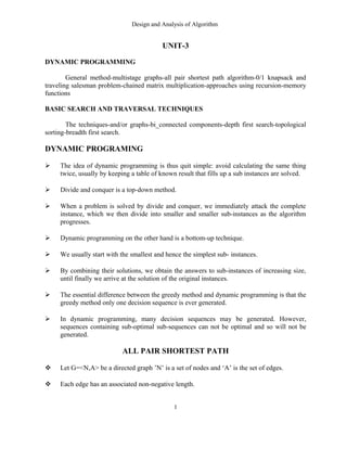
15
30
5
3
4. Design and Analysis of Algorithm
5 50 5 15
15
Fig: floyd’s algorithm and work
likewise we have to find the value for N iteration (ie)
for N nodes.
0 5 20 10 P[1,3] = 2
D2= 50 0 15 5 P[1,4] = 2
30 35 0 15
15 20 5 0
0 5 20 10
D3= 45 0 15 5 P[2,1]=3
30 35 0 15
15 20 5 0
0 5 15 10
20 0 10 5 P[1,3]=4
D4= 30 35 0 15 P[2,3]=4
15 20 5 0
D4 will give the shortest distance between any pair of
nodes.
If you want the exact path then we have to refer the
matrix p.The matrix will be,
0 0 4 2
3 0 4 0 0 direct path
P= 0 1 0 0
0 1 0 0
4
5. Design and Analysis of Algorithm
Since,p[1,3]=4,the shortest path from 1 to3 passes
through 4.
Looking now at p[1,4]&p[4,3] we discover that
between 1 & 4, we have to go to node 2 but that from 4 to 3 we proceed directly.
Finally we see the trips from 1 to 2, & from 2 to 4,
are also direct.
The shortest path from 1 to 3 is 1,2,4,3.
ALGORITHM :
Function Floyd (L[1..r,1..r]):array[1..n,1..n]
array D[1..n,1..n]
D = L
For k = 1 to n do
For i = 1 to n do
For j = 1 to n do
D [ i , j ] = min (D[ i, j ], D[ i, k ] + D[ k, j ]
Return D
ANALYSIS:
This algorithm takes a time of θ (n3
)
MULTISTAGE GRAPH
1. A multistage graph G = (V,E) is a directed graph in which the vertices are portioned
into K > = 2 disjoint sets Vi, 1 <= i<= k.
2. In addition, if < u,v > is an edge in E, then u < = Vi and V ∑ Vi+1 for some i, 1<= i < k.
3. If there will be only one vertex, then the sets Vi and Vk are such that [Vi]=[Vk] = 1.
4. Let ‘s’ and ‘t’ be the source and destination respectively.
5. The cost of a path from source (s) to destination (t) is the sum of the costs of the edger
on the path.
6. The MULTISTAGE GRAPH problem is to find a minimum cost path from ‘s’ to ‘t’.
7. Each set Vi defines a stage in the graph. Every path from ‘s’ to ‘t’ starts in stage-1, goes
to stage-2 then to stage-3, then to stage-4, and so on, and terminates in stage-k.
8. This MULISTAGE GRAPH problem can be solved in 2 ways.
a) Forward Method.
b) Backward Method.
5
6. Design and Analysis of Algorithm
FORWARD METHOD
1. Assume that there are ‘k’ stages in a graph.
2. In this FORWARD approach, we will find out the cost of each and every node starling
from the ‘k’ th
stage to the 1st
stage.
3. We will find out the path (i.e.) minimum cost path from source to the destination (ie)
[ Stage-1 to Stage-k ].
PROCEDURE:
V1 V2 V3 V4 V5
4 6
2 2
5 4
9 1
4
7 3 2
7 t
s
3
11 5 5
2
11 6
8
Maintain a cost matrix cost (n) which stores the distance from any vertex to the
destination.
If a vertex is having more than one path, then we have to choose the minimum distance
path and the intermediate vertex, which gives the minimum distance path, will be stored
in the distance array ‘D’.
In this way we will find out the minimum cost path from each and every vertex.
Finally cost(1) will give the shortest distance from source to destination.
6
7. Design and Analysis of Algorithm
For finding the path, start from vertex-1 then the distance array D(1) will give the
minimum cost neighbour vertex which in turn give the next nearest vertex and proceed
in this way till we reach the Destination.
For a ‘k’ stage graph, there will be ‘k’ vertex in the path.
In the above graph V1…V5 represent the stages. This 5 stage graph can be solved by
using forward approach as follows,
STEPS: - DESTINATION, D
Cost (12)=0 D (12)=0
Cost (11)=5 D (11)=12
Cost (10)=2 D (10)=12
Cost ( 9)=4 D ( 9)=12
For forward approach,
Cost (i,j) = min {C (j,l) + Cost (i+1,l) }
l ∈ Vi + 1
(j,l) ∈E
Cost(8) = min {C (8,10) + Cost (10), C (8,11) + Cost (11) }
= min (5 + 2, 6 + 5)
= min (7,11)
= 7
cost(8) =7 =>D(8)=10
cost(7) = min(c (7,9)+ cost(9),c (7,10)+ cost(10))
(4+4,3+2)
= min(8,5)
= 5
cost(7) = 5 =>D(7) = 10
cost(6) = min (c (6,9) + cost(9),c (6,10) +cost(10))
= min(6+4 , 5 +2)
= min(10,7)
= 7
cost(6) = 7 =>D(6) = 10
cost(5) = min (c (5,7) + cost(7),c (5,8) +cost(8))
= min(11+5 , 8 +7)
= min(16,15)
= 15
cost(5) = 15 =>D(5) = 18
cost(4) = min (c (4,8) + cost(8))
7
8. Design and Analysis of Algorithm
= min(11+7)
= 18
cost(4) = 18 =>D(4) = 8
cost(3) = min (c (3,6) + cost(6),c (3,7) +cost(7))
= min(2+7 , 7 +5)
= min(9,12)
= 9
cost(3) = 9 =>D(3) = 6
cost(2) = min (c (2,6) + cost(6),c (2,7) +cost(7) ,c (2,8) +cost(8))
= min(4+7 , 2+5 , 1+7 )
= min(11,7,8)
= 7
cost(2) = 7 =>D(2) = 7
cost(1) = min (c (1,2)+cost(2) ,c (1,3)+cost(3) ,c (1,4)+cost(4) ,c(1,5)+cost(5))
= min(9+7 , 7 +9 , 3+18 , 2+15)
= min(16,16,21,17)
= 16
cost(1) = 16 =>D(1) = 2
The path through which you have to find the shortest distance.
(i.e.)
Start from vertex - 2
D ( 1) = 2
D ( 2) = 7
D ( 7) = 10
D (10) = 12
So, the minimum –cost path is,
9 2 3 2
∴ The cost is 9+2+3+2+=16
8
9. Design and Analysis of Algorithm
ALGORITHM: FORWARD METHOD
Algorithm FGraph (G,k,n,p)
// The I/p is a k-stage graph G=(V,E) with ‘n’ vertex.
// Indexed in order of stages E is a set of edges.
// and c[i,J] is the cost of<i,j>,p[1:k] is a minimum cost path.
{
cost[n]=0.0;
for j=n-1 to 1 step-1 do
{
//compute cost[j],
// let ‘r’ be the vertex such that <j,r> is an edge of ‘G’ &
// c[j,r]+cost[r] is minimum.
cost[j] = c[j+r] + cost[r];
d[j] =r;
}
// find a minimum cost path.
P[1]=1;
P[k]=n;
For j=2 to k-1 do
P[j]=d[p[j-1]];
}
ANALYSIS:
The time complexity of this forward method is O( V + E )
BACKWARD METHOD
if there one ‘K’ stages in a graph using back ward approach. we will find out the cost of
each & every vertex starting from 1st
stage to the kth
stage.
We will find out the minimum cost path from destination to source (ie)[from stage k to
stage 1]
PROCEDURE:
1. It is similar to forward approach, but differs only in two or three ways.
2. Maintain a cost matrix to store the cost of every vertices and a distance matrix to store
the minimum distance vertex.
3. Find out the cost of each and every vertex starting from vertex 1 up to vertex k.
4. To find out the path star from vertex ‘k’, then the distance array D (k) will give the
minimum cost neighbor vertex which in turn gives the next nearest neighbor vertex and
proceed till we reach the destination.
9
11. Design and Analysis of Algorithm
D(6) = 3
D(3) = 1
So the minimum cost path is,
1 7
3 2
6 5
10 2
12
The cost is 16.
ALGORITHM : BACKWARD METHOD
Algorithm BGraph (G,k,n,p)
// The I/p is a k-stage graph G=(V,E) with ‘n’ vertex.
// Indexed in order of stages E is a set of edges.
// and c[i,J] is the cost of<i,j>,p[1:k] is a minimum cost path.
{
bcost[1]=0.0;
for j=2 to n do
{
//compute bcost[j],
// let ‘r’ be the vertex such that <r,j> is an edge of ‘G’ &
// bcost[r]+c[r,j] is minimum.
bcost[j] = bcost[r] + c[r,j];
d[j] =r;
}
// find a minimum cost path.
P[1]=1;
P[k]=n;
For j= k-1 to 2 do
P[j]=d[p[j+1]];
}
TRAVELLING SALESMAN PROBLEM
Let G(V,E) be a directed graph with edge cost cij is defined such that cij >0 for all i and j
and cij =∝ ,if <i,j> ∉ E.
Let V =n and assume n>1.
The traveling salesman problem is to find a tour of minimum cost.
A tour of G is a directed cycle that include every vertex in V.
The cost of the tour is the sum of cost of the edges on the tour.
The tour is the shortest path that starts and ends at the same vertex (ie) 1.
11
12. Design and Analysis of Algorithm
APPLICATION :
1. Suppose we have to route a postal van to pick up mail from the mail boxes located at ‘n’
different sites.
2. An n+1 vertex graph can be used to represent the situation.
3. One vertex represent the post office from which the postal van starts and return.
4. Edge <i,j> is assigned a cost equal to the distance from site ‘i’ to site ‘j’.
5. the route taken by the postal van is a tour and we are finding a tour of minimum length.
6. every tour consists of an edge <1,k> for some k ∈ V-{} and a path from vertex k to
vertex 1.
7. the path from vertex k to vertex 1 goes through each vertex in V-{1,k} exactly once.
8. the function which is used to find the path is
g(1,V-{1}) = min{ cij + g(j,s-{j})}
9. g(i,s) be the length of a shortest path starting at vertex i, going
through all vertices in S,and terminating at vertex 1.
10. the function g(1,v-{1}) is the length of an optimal tour.
STEPS TO FIND THE PATH:
1. Find g(i,Φ) =ci1, 1<=i<n, hence we can use equation(2) to obtain g(i,s) for all s to size 1.
2. That we have to start with s=1,(ie) there will be only one vertex in set ‘s’.
3. Then s=2, and we have to proceed until |s| <n-1.
4. for example consider the graph.
10
15
10
15
20 8 9 13
8 6
12
7
Cost matrix
0 10 15 20
5 0 9 10
6 13 0 12
8 8 9 0
12
13. Design and Analysis of Algorithm
g(i,s) set of nodes/vertex have to visited.
starting position
g(i,s) =min{cij +g(j,s-{j})
STEP 1:
g(1,{2,3,4})=min{c12+g(2{3,4}),c13+g(3,{2,4}),c14+g(4,{2,3})}
min{10+25,15+25,20+23}
min{35,35,43}
=35
STEP 2:
g(2,{3,4}) = min{c23+g(3{4}),c24+g(4,{3})}
min{9+20,10+15}
min{29,25}
=25
g(3,{2,4}) =min{c32+g(2{4}),c34+g(4,{2})}
min{13+18,12+13}
min{31,25}
=25
g(4,{2,3}) = min{c42+g(2{3}),c43+g(3,{2})}
min{8+15,9+18}
min{23,27}
=23
STEP 3:
1. g(3,{4}) = min{c34 +g{4,Φ}}
12+8 =20
2. g(4,{3}) = min{c43 +g{3,Φ}}
9+6 =15
3. g(2,{4}) = min{c24 +g{4,Φ}}
13
15. Design and Analysis of Algorithm
g(3,{4}) = c34 + g(4,Φ)
= 12+8 =20
g(4,{2}) = c42 + g(2,Φ)
= 8+5 =13
g(4,{3}) = c43 + g(3,Φ)
= 9+6 =15
s = 2
i ≠ 1, 1∈ s and i ∈ s.
g(2,{3,4}) = min{c23+g(3{4}),c24+g(4,{3})}
min{9+20,10+15}
min{29,25}
=25
g(3,{2,4}) =min{c32+g(2{4}),c34+g(4,{2})}
min{13+18,12+13}
min{31,25}
=25
g(4,{2,3}) = min{c42+g(2{3}),c43+g(3,{2})}
min{8+15,9+18}
min{23,27}
=23
s = 3
g(1,{2,3,4})=min{c12+g(2{3,4}),c13+g(3,{2,4}),c14+g(4,{2,3})}
min{10+25,15+25,20+23}
min{35,35,43}
=35
optimal cost is 35
the shortest path is,
g(1,{2,3,4}) = c12 + g(2,{3,4}) => 1->2
g(2,{3,4}) = c24 + g(4,{3}) => 1->2->4
g(4,{3}) = c43 + g(3{Φ}) => 1->2->4->3->1
15
16. Design and Analysis of Algorithm
so the optimal tour is 1 2 4 3 1
CHAINED MATRIX MULTIPLICATION:
If we have a matrix A of size p×q and B matrix of size q×r.the product of these two matrix C is
given by,
cij = Σ aik bkj , 1≤ i ≤ p, 1≤ j ≤ r , 1= k =q.
it requires a total of pqr scalar multiplication.
Matrix multiplication is associative, so if we want to calculate the product of more then 2
matrixes m= m1m2… mn.
For example,
A = 13 × 5
B = 5 × 89
C = 89 × 3
D = 3 × 34
Now, we will see some of the sequence,
M = (((A.B).C).D)
A.B C
= (13 * 5 * 89) * (89 * 3)
A.B.C. D
= (13 * 89 * 3) * (3 * 34)
A.B.C.D
= 13 * 3 * 34
(ic) = 13 * 5 * 89 + 13 * 89 * 3 + 13 * 3 * 34
= 10,582 no. of multiplications one required for that
sequence.
2nd
Sequence,
M = (A * B) * (C * D)
= 13 * 5 * 89 + 89 * 3 * 34 + 13 * 89 * 34
= 54201 no. of Multiplication
3rd
Sequence,
16
17. Design and Analysis of Algorithm
M = (A.(BC)) . D
= 5 * 89 * 3 + 13 * 5 * 3 + 13 * 3 *34
= 2856
For comparing all these sequence, (A(BC)).D sequences less no. of multiplication.
For finding the no. of multiplication directly, we are going to the Dynamic programming
method.
STRAIGHT FORWARD METHOD:
Our aim is to find the total no. of scalar multiplication required to compute the matrix product.
Let (M1,M2,……Mi) and Mi+1,Mi+2,……Mn be the chain of matrix to be calculated using
the dynamic programming method.
In dynamic programming, we always start with the smallest instances and continue till we
reach the required size.
We maintain a table mij, 1≤ i ≤ j≤ n,
Where mij gives the optimal solution.
Sizes of all the matrixes are stored in the array d[0..n]
We build the table diagonal by diagonal; diagonal s contains the elements mij such that j-1 =s.
RULES TO FILL THE TABLE Mij:
S =0,1,……n-1
If s=0 => m(i,i) =0 ,i =1,2,……n
If s=1 => m(i,i+1) = d(i-1)*di *d(i+1)
i=1,2,……n-1.
If 1< s <n =>mi,i+s =min(mik+mk+1,i+s+di-1dkdi+s)
i≤ k ≤ i+s i = 1,2,……n-s
apply this to the example,
A=>13×5
B=>5×89
C=>89×3
D=>3×34
Single dimension array is used to store the sizes.
17
19. Design and Analysis of Algorithm
2 0 1335 1845 s=2
3 0 9078 s=1
4 0 s=0
No need to fill the lower diagonal
ALGORITHM:
Procedure cmatrix(n,d[0..n])
For s=0 to n-1 do
{
if(s==0)
for I=1 ton do
m(i,j) =0
if(s==1)
for i=1 to n-1 do
m(i,i+1) =d(i-1)*d(i)*d(i+1)
else
{
m=∝
for i=1 to n-s do
for k=i to i+s do
{
if (min>[m(i,k) +m(k+1,i+s)+d(i-1)*d(k)*d(i+s)])
min=[m(i,k) +m(k+1,i+s)+d(i-1)*d(k)*d(i+s)]
}
m(i,i+s) =min
}
}
0/1 KNAPSACK PROBLEM:
This problem is similar to ordinary knapsack problem but we may not take a fraction of
an object.
We are given ‘ N ‘ object with weight Wi and profits Pi where I varies from l to N and
also a knapsack with capacity ‘ M ‘.
The problem is, we have to fill the bag with the help of ‘ N ‘ objects and the resulting
profit has to be maximum.
19
20. Design and Analysis of Algorithm
n
Formally, the problem can be started as, maximize ∑ Xi Pi
i=l
n
subject to ∑ Xi Wi L M
i=l
Where Xi are constraints on the solution Xi ∈{0,1}. (u) Xi is required to be 0 or 1. if the
object is selected then the unit in 1. if the object is rejected than the unit is 0. That is
why it is called as 0/1, knapsack problem.
To solve the problem by dynamic programming we up a table T[1…N, 0…M] (ic) the
size is N. where ‘N’ is the no. of objects and column starts with ‘O’ to capacity (ic) ‘M’.
In the table T[i,j] will be the maximum valve of the objects i varies from 1 to n and j
varies from O to M.
RULES TO FILL THE TABLE:-
If i=l and j < w(i) then T(i,j) =o, (ic) o pre is filled in the table.
If i=l and j ≥ w (i) then T (i,j) = p(i), the cell is filled with the profit p[i], since only one
object can be selected to the maximum.
If i>l and j < w(i) then T(i,l) = T (i-l,j) the cell is filled the profit of previous object
since it is not possible with the current object.
If i>l and j ≥ w(i) then T (i,j) = {f(i) +T(i-l,j-w(i)),. since only ‘l’ unit can be selected to
the maximum. If is the current profit + profit of the previous object to fill the remaining
capacity of the bag.
After the table is generated, it will give details the profit.
ES TO GET THE COMBINATION OF OBJECT:
Start with the last position of i and j, T[i,j], if T[i,j] = T[i-l,j] then no object of ‘i’ is
required so move up to T[i-l,j].
After moved, we have to check if, T[i,j]=T[i-l,j-w(i)]+ p[I], if it is equal then one unit of
object ‘i’ is selected and move up to the position T[i-l,j-w(i)]
Repeat the same process until we reach T[i,o], then there will be nothing to fill the bag
stop the process.
20
21. Design and Analysis of Algorithm
Time is 0(nw) is necessary to construct the table T.
Consider a Example,
M = 6,
N = 3
W1 = 2, W2 = 3, W3 = 4
P1 = 1, P2 =2, P3 = 5
i 1 to N
j 0 to 6
i=l, j=o (ic) i=l & j < w(i)
o<2 T1,o =0
i=l, j=l (ic) i=l & j < w(i)
l<2 T1,1 =0 (Here j is equal to w(i) P(i)
i=l, j=2
2 o,= T1,2 = l.
i=l, j=3
3>2,= T1,3 = l.
i=l, j=4
4>2,= T1,4 = l.
i=l, j=5
5>2,= T1,5 = l.
i=l, j=6
6>2,= T1,6 = l.
=> i=2, j=o (ic) i>l,j<w(i)
o<3= T(2,0) = T(i-l,j) = T(2)
T 2,0 =0
i=2, j=1
l<3= T(2,1) = T(i-l)
T 2,1 =0
BASIC SEARCH AND TRAVERSAL TECHNIQUE:
21
22. Design and Analysis of Algorithm
GRAPH
DEFINING GRAPH:
A graphs g consists of a set V of vertices (nodes) and a set E of edges (arcs). We
write G=(V,E). V is a finite and non-empty set of vertices. E is a set of pair of vertices; these
pairs are called as edges . Therefore,
V(G).read as V of G, is a set of vertices and E(G),read as E of G is a set of edges.
An edge e=(v, w) is a pair of vertices v and w, and to be incident with v and w.
A graph can be pictorially represented as follows,
FIG: Graph G
We have numbered the graph as 1,2,3,4. Therefore, V(G)=(1,2,3,4) and
E(G) = {(1,2),(1,3),(1,4),(2,3),(2,4)}.
BASIC TERMINOLGIES OF GRAPH:
UNDIRECTED GRAPH:
An undirected graph is that in which, the pair of vertices representing the edges is
unordered.
DIRECTED GRAPH:
An directed graph is that in which, each edge is an ordered pair of vertices, (i.e.)
each edge is represented by a directed pair. It is also referred to as digraph.
DIRECTED GRAPH
COMPLETE GRAPH:
An n vertex undirected graph with exactly n(n-1)/2 edges is said to be complete
graph. The graph G is said to be complete graph .
22
1
2 3
4
23. Design and Analysis of Algorithm
TECHNIQUES FOR GRAPHS:
The fundamental problem concerning graphs is the reach-ability problem.
In it simplest from it requires us to determine whether there exist a path in the given
graph, G +(V,E) such that this path starts at vertex ‘v’ and ends at vertex ‘u’.
A more general form is to determine for a given starting vertex v6 V all vertex ‘u’ such
that there is a path from if it u.
This problem can be solved by starting at vertex ‘v’ and systematically searching the
graph ‘G’ for vertex that can be reached from ‘v’.
We describe 2 search methods for this.
i. Breadth first Search and Traversal.
ii. Depth first Search and Traversal.
BREADTH FIRST SEARCH AND TRAVERSAL:
Breadth first search:
In Breadth first search we start at vertex v and mark it as having been reached. The
vertex v at this time is said to be unexplored. A vertex is said to have been explored by an
algorithm when the algorithm has visited all vertices adjacent from it. All unvisited vertices
adjacent from v are visited next. There are new unexplored vertices. Vertex v has now been
explored. The newly visited vertices have not been explored and are put onto the end of the list
of unexplored vertices. The first vertex on this list is the next to be explored. Exploration
continues until no unexplored vertex is left. The list of unexplored vertices acts as a queue and
can be represented using any of the standard queue representations.
In Breadth First Search we start at a vertex ‘v’ and mark it as having been reached
(visited).
The vertex ‘v’ is at this time said to be unexplored.
A vertex is said to have been explored by an algorithm when the algorithm has visited
all vertices adjust from it.
All unvisited vertices adjust from ‘v’ are visited next. These are new unexplored
vertices.
Vertex ‘v’ has now been explored. The newly visit vertices have not been explored and
are put on the end of a list of unexplored vertices.
The first vertex on this list in the next to be explored. Exploration continues until no
unexplored vertex is left.
The list of unexplored vertices operates as a queue and can be represented using any of
the start queue representation.
ALGORITHM:
Algorithm BPS (v)
23
24. Design and Analysis of Algorithm
// A breadth first search of ‘G’ is carried out.
// beginning at vertex-v; For any node i, visit.
// if ‘i’ has already been visited. The graph ‘v’
// and array visited [] are global; visited []
// initialized to zero.
{ y=v; // q is a queue of unexplored 1visited (v)= 1
repeat
{ for all vertices ‘w’ adjacent from u do
{ if (visited[w]=0) then
{Add w to q;
visited[w]=1
}
}
if q is empty then return;// No delete u from q;
} until (false)
}
algrothim : breadth first traversal
algorithm BFT(G,n)
{
for i= 1 to n do
visited[i] =0;
for i =1 to n do
if (visited[i]=0)then BFS(i)
}
here the time and space required by BFT on an n-vertex e-edge graph one O(n+e) and O(n) resp
if adjacency list is used.if adjancey matrix is used then the bounds are O(n2
) and O(n) resp
DEPTH FIRST SEARCH
A depth first search of a graph differs from a breadth first search in that the exploration
of a vertex v is suspended as soon as a new vertex is reached. At this time the exploration of the
new vertex u begins. When this new vertex has been explored, the exploration of u continues.
The search terminates when all reached vertices have been fully explored. This search process
is best-described recursively.
Algorithm DFS(v)
{
visited[v]=1
for each vertex w adjacent from v do
{
If (visited[w]=0)then
24
25. Design and Analysis of Algorithm
DFS(w);
}
}
TOPOLOGICAL SORT
A topological sort of a DAG G is an ordering of the vertices of G such that for every
edge (ei, ej) of G we have i<j. That is, a topological sort is a linear ordering of all its vertices
such that if DAG G contains an edge (ei, ej), then ei appears before ej in the ordering. DAG is
cyclic then no linear ordering is possible.
In simple words, a topological ordering is an ordering such that any directed path in DAG G
traverses vertices in increasing order.
It is important to note that if the graph is not acyclic, then no linear ordering is possible. That is,
we must not have circularities in the directed graph. For example, in order to get a job you need
to have work experience, but in order to get work experience you need to have a job.
Theorem: A directed graph has a topological ordering if and only if it is acyclic.
Proof:
Part 1. G has a topological ordering if is G acyclic.
Let G is topological order.
Let G has a cycle (Contradiction).
Because we have topological ordering. We must have i0, < i, < . . . < ik-1 < i0, which is clearly
impossible.
Therefore, G must be acyclic.
Part 2. G is acyclic if has a topological ordering.
Let is G acyclic.
Since is G acyclic, must have a vertex with no incoming edges. Let v1 be such a vertex. If we
remove v1 from graph, together with its outgoing edges, the resulting digraph is still acyclic.
Hence resulting digraph also has a vertex *
ALGORITHM: TOPOLOGICAL_SORT(G)
1. For each vertex find the finish time by calling DFS(G).
2. Insert each finished vertex into the front of a linked list.
3. Return the linked list.
Example:
25
26. Design and Analysis of Algorithm
1. given graph G; start node u
Diagram
with no incoming edges, and we let v2 be such a vertex. By repeating this process until digraph
G becomes empty, we obtain an ordering v1<v2 < , . . . , vn of vertices of digraph G. Because of
the construction, if (vi, vj) is an edge of digraph G, then vi must be detected before vj can be
deleted, and thus i<j. Thus, v1, . . . , vn is a topological sorting.
Total running time of topological sort is θ(V+E) . Since DFS(G) search takes θ(V+E) time and
it takes O(1) time to insert each of the |V| vertices onto the front of the linked list.
26