Eigen Decomposition

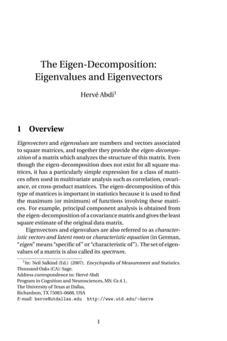
1. The Eigen-Decomposition:
Eigenvalues and Eigenvectors
Hervé Abdi1
1 Overview
Eigenvectors and eigenvalues are numbers and vectors associated
to square matrices, and together they provide the eigen-decompo-
sition of a matrix which analyzes the structure of this matrix. Even
though the eigen-decomposition does not exist for all square ma-
trices, it has a particularly simple expression for a class of matri-
ces often used in multivariate analysis such as correlation, covari-
ance, or cross-product matrices. The eigen-decomposition of this
type of matrices is important in statistics because it is used to find
the maximum (or minimum) of functions involving these matri-
ces. For example, principal component analysis is obtained from
the eigen-decomposition of a covariance matrix and gives the least
square estimate of the original data matrix.
Eigenvectors and eigenvalues are also referred to as character-
istic vectors and latent roots or characteristic equation (in German,
“eigen” means “specific of” or “characteristic of”). The set of eigen-
values of a matrix is also called its spectrum.
1
In: Neil Salkind (Ed.) (2007). Encyclopedia of Measurement and Statistics.
Thousand Oaks (CA): Sage.
Address correspondence to: Hervé Abdi
Program in Cognition and Neurosciences, MS: Gr.4.1,
The University of Texas at Dallas,
Richardson, TX 75083–0688, USA
E-mail: herve@utdallas.edu http://www.utd.edu/∼herve
1

2. Hervé Abdi: The Eigen-Decomposition
3
2
12
8
u1
1
Au
-1
1
1
-1
u
Au
a b
2
2
Figure 1: Two eigenvectors of a matrix.
2 Notations and definition
There are several ways to define eigenvectors and eigenvalues, the
most common approach defines an eigenvector of the matrix A as
a vector u that satisfies the following equation:
Au = λu . (1)
when rewritten, the equation becomes:
(A−λI)u = 0 , (2)
where λ is a scalar called the eigenvalue associated to the eigenvec-
tor.
In a similar manner, we can also say that a vector u is an eigen-
vector of a matrix A if the length of the vector (but not its direction)
is changed when it is multiplied by A.
For example, the matrix:
A =
·
2 3
2 1
¸
(3)
has the eigenvectors:
u1 =
·
3
2
¸
with eigenvalue λ1 = 4 (4)
2

3. Hervé Abdi: The Eigen-Decomposition
and
u2 =
·
−1
1
¸
with eigenvalue λ2 = −1 (5)
We can verify (as illustrated in Figure 1) that only the length of u1
and u2 is changed when one of these two vectors is multiplied by
the matrix A:
·
2 3
2 1
¸·
3
2
¸
= 4
·
3
2
¸
=
·
12
8
¸
(6)
and
·
2 3
2 1
¸·
−1
1
¸
= −1
·
−1
1
¸
=
·
1
−1
¸
. (7)
For most applications we normalize the eigenvectors (i.e., trans-
form them such that their length is equal to one):
uT
u = 1 . (8)
For the previous example we obtain:
u1 =
·
.8331
.5547
¸
. (9)
We can check that:
·
2 3
2 1
¸·
.8331
.5547
¸
=
·
3.3284
2.2188
¸
= 4
·
.8331
.5547
¸
(10)
and ·
2 3
2 1
¸·
−.7071
.7071
¸
=
·
.7071
−.7071
¸
= −1
·
−.7071
.7071
¸
. (11)
Traditionally, we put together the set of eigenvectors of A in a ma-
trix denoted U. Each column of U is an eigenvector of A. The
eigenvalues are stored in a diagonal matrix (denoted Λ), where the
diagonal elements gives the eigenvalues (and all the other values
are zeros). We can rewrite the first equation as:
AU = UΛ ; (12)
3

4. Hervé Abdi: The Eigen-Decomposition
or also as:
A = UΛU−1
. (13)
For the previous example we obtain:
A = UΛU−1
=
·
3 −1
2 1
¸·
4 0
0 −1
¸·
.2 .2
−.4 .6
¸
=
·
2 3
2 1
¸
. (14)
It is important to note that not all matrices have eigenvalues.
For example, the matrix
·
0 1
0 0
¸
does not have eigenvalues. Even
when a matrix has eigenvalues and eigenvectors, the computation
of the eigenvectors and eigenvalues of a matrix requires a large
number of computations and is therefore better performed by com-
puters.
2.1 Digression:
An infinity of eigenvectors for one eigenvalue
It is only through a slight abuse of language that we can talk about
the eigenvector associated with one given eigenvalue. Strictly speak-
ing, there is an infinity of eigenvectors associated to each eigen-
value of a matrix. Because any scalar multiple of an eigenvector is
still an eigenvector, there is, in fact, an (infinite) family of eigen-
vectors for each eigenvalue, but they are all proportional to each
other. For example, ·
1
−1
¸
(15)
is an eigenvector of the matrix A:
·
2 3
2 1
¸
. (16)
4

5. Hervé Abdi: The Eigen-Decomposition
Therefore:
2×
·
1
−1
¸
=
·
2
−2
¸
(17)
is also an eigenvector of A:
·
2 3
2 1
¸·
2
−2
¸
=
·
−2
2
¸
= −1×2
·
1
−1
¸
. (18)
3 Positive (semi-)definite matrices
A type of matrices used very often in statistics are called positive
semi-definite. The eigen-decomposition of these matrices always
exists, and has a particularly convenient form. A matrix is said to
be positive semi-definite when it can be obtained as the product of
a matrix by its transpose. This implies that a positive semi-definite
matrix is always symmetric. So, formally, the matrix A is positive
semi-definite if it can be obtained as:
A = XXT
(19)
for a certain matrix X (containing real numbers). Positive semi-
definite matrices of special relevance for multivariate analysis pos-
itive semi-definite matrices include correlation matrices. covari-
ance, and, cross-product matrices.
The important properties of a positive semi-definite matrix is
that its eigenvalues are always positive or null, and that its eigen-
vectors are pairwise orthogonal when their eigenvalues are differ-
ent. The eigenvectors are also composed of real values (these last
two properties are a consequence of the symmetry of the matrix,
for proofs see, e.g., Strang, 2003; or Abdi & Valentin, 2006). Be-
cause eigenvectors corresponding to different eigenvalues are or-
thogonal, it is possible to store all the eigenvectors in an orthogo-
nal matrix (recall that a matrix is orthogonal when the product of
this matrix by its transpose is a diagonal matrix).
This implies the following equality:
U−1
= UT
. (20)
5

6. Hervé Abdi: The Eigen-Decomposition
We can, therefore, express the positive semi-definite matrix A as:
A = UΛUT
(21)
where UTU = I are the normalized eigenvectors; if they are not
normalized then UTU is a diagonal matrix.
For example, the matrix:
A =
·
3 1
1 3
¸
(22)
can be decomposed as:
A = UΛUT
=


q
1
2
q
1
2
q
1
2 −
q
1
2


·
4 0
0 2
¸


q
1
2
q
1
2
q
1
2 −
q
1
2


=
·
3 1
1 3
¸
, (23)
with 

q
1
2
q
1
2
q
1
2
−
q
1
2




q
1
2
q
1
2
q
1
2
−
q
1
2

 =
·
1 0
0 1
¸
. (24)
3.1 Diagonalization
When a matrix is positive semi-definite we can rewrite Equation
21 as
A = UΛUT
⇐⇒ Λ = UT
AU . (25)
This shows that we can transform the matrix A into an equivalent
diagonal matrix. As a consequence, the eigen-decomposition of a
positive semi-definite matrix is often referred to as its diagonaliza-
tion.
6

7. Hervé Abdi: The Eigen-Decomposition
3.2 Another definition for positive semi-definite ma-
trices
A matrix A is said to be positive semi-definite if we observe the
following relationship for any non-zero vector x:
xT
Ax ≥ 0 ∀x . (26)
(when the relationship is ≤ 0 we say that the matrix is negative
semi-definite).
When all the eigenvalues of a symmetric matrix are positive,
we say that the matrix is positive definite. In that case, Equation 26
becomes:
xT
Ax > 0 ∀x . (27)
4 Trace, Determinant, etc.
The eigenvalues of a matrix are closely related to three important
numbers associated to a square matrix, namely its trace, its deter-
minant and its rank.
4.1 Trace
The trace of a matrix A is denoted trace{A} and is equal to the sum
of its diagonal elements. For example, with the matrix:
A =


1 2 3
4 5 6
7 8 9

 (28)
we obtain:
trace{A} = 1+5+9 = 15 . (29)
The trace of a matrix is also equal to the sum of its eigenvalues:
trace{A} =
X
`
λ` = trace{Λ} (30)
with Λ being the matrix of the eigenvalues of A. For the previous
example, we have:
Λ = diag{16.1168,−1.1168,0} . (31)
7

8. Hervé Abdi: The Eigen-Decomposition
We can verify that:
trace{A} =
X
`
λ` = 16.1168+(−1.1168) = 15 (32)
4.2 Determinant and rank
Another classic quantity associated to a square matrix is its deter-
minant. This concept of determinant, which was originally de-
fined as a combinatoric notion, plays an important rôle in com-
puting the inverse of a matrix and in finding the solution of sys-
tems of linear equations (the term determinant is used because
this quantity determines the existence of a solution in systems of
linear equations). The determinant of a matrix is also equal to the
product of its eigenvalues. Formally, if |A| the determinant of A, we
have:
|A| =
Y
`
λ` with λ` being the `-th eigenvalue of A . (33)
For example, the determinant of matrix A (from the previous sec-
tion), is equal to:
|A| = 16.1168×−1.1168×0 = 0 . (34)
Finally, the rank of a matrix can be defined as being the num-
ber of non-zero eigenvalues of the matrix. For our example:
rank{A} = 2 . (35)
For a positive semi-definite matrix, the rank corresponds to the
dimensionality of the Euclidean space which can be used to rep-
resent the matrix. A matrix whose rank is equal to its dimensions
is called a full rank matrix. When the rank of a matrix is smaller
than its dimensions, the matrix is called rank-deficient, singular,
or multicolinear. Only full rank matrices have an inverse.
5 Statistical properties of
the eigen-decomposition
The eigen-decomposition is important because it is involved in
problems of optimization. For example, in principal component
8

9. Hervé Abdi: The Eigen-Decomposition
analysis, we want to analyze an I × J matrix X where the rows are
observations and the columns are variables describing these ob-
servations. The goal of the analysis is to find row factor scores,
such that these factor scores “explain” as much of the variance of
X as possible, and such that the sets of factor scores are pairwise
orthogonal. This amounts to defining the factor score matrix as
F = XP , (36)
under the constraints that
FT
F = PT
XT
XP (37)
is a diagonal matrix (i.e., F is an orthogonal matrix) and that
PT
P = I (38)
(i.e., P is an orthonormal matrix). There are several ways of obtain-
ing the solution of this problem. One possible approach is to use
the technique of the Lagrangian multipliers where the constraint
from Equation 38 is expressed as the multiplication with a diago-
nal matrix of Lagrangian multipliers denoted Λ in order to give the
following expression
Λ
³
PT
P−I
´
(39)
(see Harris, 2001; and Abdi & Valentin, 2006; for details). This
amount to defining the following equation
L = FT
F−Λ
³
PT
P−I
´
= PT
XT
XP−Λ
³
PT
P−I
´
. (40)
In order to find the values of P which give the maximum values of
L , we first compute the derivative of L relative to P:
∂L
∂P
= 2XT
XP−2ΛP, (41)
and then set this derivative to zero:
XT
XP−ΛP = 0 ⇐⇒ XT
XP = ΛP . (42)
9

10. Hervé Abdi: The Eigen-Decomposition
Because Λ is diagonal, this is clearly an eigen-decomposition prob-
lem, and this indicates that Λ is the matrix of eigenvalues of the
positive semi-definite matrix XTX ordered from the largest to the
smallest and that P is the matrix of eigenvectors of XTX associated
to Λ. Finally, we find that the factor matrix has the form
F = PΛ
1
2 . (43)
The variance of the factors scores is equal to the eigenvalues:
FT
F = Λ
1
2 PT
PΛ
1
2 = Λ . (44)
Taking into account that the sum of the eigenvalues is equal to
the trace of XTX, this shows that the first factor scores “extract”
as much of the variances of the original data as possible, and that
the second factor scores extract as much of the variance left un-
explained by the first factor, and so on for the remaining factors.
Incidently, the diagonal elements of the matrix Λ
1
2 which are the
standard deviations of the factor scores are called the singular val-
ues of matrix X (see entry on singular value decomposition).
References
[1] Abdi, H. (2003). Multivariate analysis. In M. Lewis-Beck, A. Bry-
man, & T. Futing (Eds): Encyclopedia for research methods for
the social sciences. Thousand Oaks: Sage.
[2] Abdi, H., Valentin, D. (2006). Mathématiques pour les sciences
cognitives (Mathematics for cognitive sciences). Grenoble: PUG.
[3] Harris, R.j. (2001). A primer of multivariate statistics. Mahwah
(NJ): Erlbaum.
[4] Strang, G. (2003). Introduction to linear algebra. Cambridge
(MA): Wellesley-Cambridge Press.
10