SlideShare ist ein Scribd-Unternehmen logo
1 von 133
MACROECONOMICS & BUSINESS ENVIRONMENT
(SLEC502 – Semester II)
Lecture Notes (Session 1 to 10)
Chapter 1-Introduction to economic Analysis (Session 1)
Microeconomics:-
1. It is the study of individual economic units of an economy.
2. It deals with Individual Income, Individual prices, Individual output, etc.
3. Its central problem is price determination and allocation of resources.
4. Its main tools are demand and supply of a particular commodity/factor.
5. It helps to solve the central problem of ‘what, how and for whom’ to produce. In the
economy
6. It discusses how equilibrium of a consumer, a producer or an Industry Is attained.
7. Price is the main determinant of micro- economic problems.
8. Examples are: Individual Income, Individual savings, price determination of a commodity,
individual firm’s output, consumer’s equilibrium.
Macroeconomics:
1. It is the study of economy as a whole and its aggregates.
2. It deals with aggregates like national Income, general price level, national output, etc.
3. Its central problem is determination of level of Income and employment.
4. Its main tools are aggregate demand and aggregate supply of the economy as a whole.
5. It helps to solve the central problem of full employment of resources in the economy.
6. It is concerned with the determination of equilibrium level of Income and employment of
the economy.
7. Income is the major determinant of macroeconomic problems.
8. Examples are: National Income, national savings, general price level, aggregate demand,
aggregate supply, poverty, unemployment, etc.
Macroeconomic Policy Objectives:
The macroeconomic policy objectives are the following:
(i) Full employment,
(ii) Price stability,
(iii) Economic growth,
(iv) Balance of payments equilibrium and exchange rate stability, and
(v) Social objectives.
(i) Full employment:
Performance of any government is judged in terms of goals of achieving full employment and
price stability. These two may be called the key indicators of health of an economy. In other
words, modern governments aim at reducing both unemployment and inflation rates.
Unemployment refers to involuntary idle-ness of mainly labour force and other produc-tive
resources. Unemployment (of labour) is closely related to the economy’s aggregate output.
Higher the unemployment rate, greater the divergence between actual aggre-gate output (or
GNP/CDP) and potential out-put. So, one of the objectives of macroeco-nomic policy is to
ensure full employment.
(ii) Price stability:
No longer the attainment of full employment is considered as a macroeconomic goal. The
emphasis has shifted to price stability. By price stability we must not mean an unchanging
price level over time. Not necessarily, price increase is unwelcome, particularly if it is
restricted within a reasonable limit. In other words, price fluc-tuations of a larger degree are
always unwelcome.
However, it is difficult again to define the permissible or reasonable rate of inflation. But
sustained increase in price level as well as a falling price level produce destabilizing effects
on the economy. Therefore, one of the objectives of macroeconomic policy is to ensure
(relative) price level stability. This goal prevents not only economic fluctuations but also
helps in the attainment of a steady growth of an economy.
(iii) Economic growth:
Economic growth in a market economy is never steady. These economies experience ups and
downs in their performance. One of the important benchmarks to measure the performance of
an economy is the rate of increase in output over a period of time. There are three major’
sources of economic growth, viz. (i) the growth of the labour force, (ii) capital formation, and
(iii) technological progress. A country seeks to achieve higher economic growth over a long
period so that the standards of living or the quality of life of people, on an average, improve.
It may be noted here that while talking about higher economic growth, it takes into account
general, social and environmental factors so that the needs of people of both present
generations and future generations can be met.
(iv) Balance of payments equilibrium and exchange rate stability:
From a macro- economic point of view, one can show that an international transaction differs
from domestic transaction in terms of (foreign) currency exchange. Over a period of time, all
countries aim at balanced flow of goods, services and assets into and out of the country.
Whenever this happens, total international monetary reserves are viewed as stable.
It is, however, because of growing inter- connectedness and interdependence between
different nations in the globalised world, the task of fulfilling this macroeconomic policy
objective has become more problematic.
(v) Social objectives:
Macroeconomic policy is also used to attain some social ends or social welfare. This means
that income distribution needs to be more fair and equitable. In a capitalist market-based
society some people get more than others. In order to ensure social justice, policymakers use
macroeconomic policy instruments.
Macroeconomic Policy Instruments:
As our macroeconomic goals are not typically confined to “full employment”, “price
stability”, “rapid growth”, “BOP equilibrium and stability in foreign exchange rate”, so our
macroeconomic policy instruments include monetary policy, fiscal policy, income policy in a
narrow sense. But, in a broder sense, these instruments should include policies relating to
labour, tariff, agriculture, anti-monopoly and other relevant ones that influence the
macroeconomic goals of a country. Confining our attention in a restricted way we intend to
consider two types of policy instruments the two “giants of the industry” monetary (credit)
policy and fiscal (budgetary) policy. These two policies are employed toward altering
aggregate demand so as to bring about a change in aggregate output (GNP/GDP) and prices,
wages and interest rates, etc., throughout the economy.
Circular Flow of Income
1. The Circular Flow of Income in a Two-Sector Model:
In this model, the economy is assumed to be a closed economy and consists of only two
sectors, i.e., the household and the firms. A closed economy is an economy that does not
participate in international trade. In this model, the household sector is the only buyer of
the goods and services produced by the firms and it is also the only supplier of the factors
of production. The household sector spends the entire income on the purchase of goods
and services produced by the firms implying that there is no saving or investment in the
economy. The firms are the only producer of the good and services. The firms generate
income by selling the goods and services to the household sector and the latter earns
income by selling the factors of production to the former. Thus, the income of the
producers is equal to the income of the households is equal to the consumption
expenditure of the household. The demand of the economy is equal to the supply. In this
model, Y = C where, Y is Income and C is Consumption. The circular flow of income in
a two sector model is explained with the help of the following diagram, called Model 1.
The Circular Flow of Income in a Two-Sector Model with Saving and Investment:
In the above model, we assumed that the household sector spends its entire income and
that there is no saving in the economy however, in practice, the household sector does not
spend all its income; it saves a part of it. The saving by the household sector would imply
monetary withdrawal (equal to saving) from the circular flow of income. This would
affect thesale of the firms since the entire income of the household would not reach the
firm implying that the production of goods and services would be more than the sale.
Consequently, the firms would decrease their production which would lead to a fall in the
income of the household and so on. There is one way of equating the sales of the firms
with the income generated; if the saving of the household is credited to the firms for
investment then the income gap could be filled. If the total investment (I) of the firms is
equal to the total saving (S) of the household sector then the equilibrium level of the
economy would be maintained at the original level. This is explained with the help of the
following diagram, called Model 1a. The equilibrium condition for a two-sector model
with saving and investment is as follows:Y = C + S or Y = C + I or C + S = C + IOr, S
= I Where, Y = Income, C = Consumption, S = Saving and I = Investment.
2. The Circular Flow of Income in a Three –Sector Model:
The three sector model of circular flow of income highlights the role played by the
government sector. This is a more realistic model which includes the economic activities
of the government however; we continue to assume the economy to be a closed one.
There are no transactions with the rest of the world. The government levies taxes on the
households and the firms and it also gives subsidies to the firms and transfer payments to
the household sector. Thus, there is income flow from the household and firmsto the
government via taxes in one direction and there is income outflow from the government
to the household and firms in the other direction. If the government revenue falls short of
its expenditure, it is also known to borrow through financial markets. This sector adds
three key elements to the circular flow model, i.e., taxes, government purchases and
government borrowings. This is explained with the help of the following diagram called,
Model 2.
In this model, the equilibrium condition is as follows:Y = C + I + GWhere, Y = Income; C =
Consumption; I = Investment and G = Government ExpenditureIn a closed economy,
aggregate demand is measured by adding consumption, investment and government
expenditure. Thus, aggregate demand is defined as the total demand for final goods and
services in an economy at a given time and price level and aggregate supply is defined as the
total supply of goods and services that the firms are willing to sell in an economy at a given
price level.
3. The Circular Flow Of Income in a Four Sector Model:
This is the complete model of the circular flow of income that incorporates all the four
macroeconomic sectors. Along with the above three sectors it considers the effect of foreign
trade on the circular flow. With the inclusion of this sector the economy now becomes an
‘open economy’. Foreign trade includes two transactions, i.e., exports and imports. Goods
and services are exported from one country to the other countries and imports come to a
country from different countries in the goods market. There is inflow of income to the firms
and government in the form of payments for the exports and there is outflow of income when
the firms and governments make payments abroad for the imports. The import payments and
export receipts transactions are done in the financial market. This is explained with the help
of a following diagram, called Model 3.
In this model, the equilibrium condition is as follows:Y = C + I + G + NX
NX = Net Exports = Exports (X) –Imports (M), Where, Y = Income; C = Consumption; I =
Investment; G = Government Expenditure; X = Exports and M = Imports.
Leakages and Injections in the Circular Flow of Income:
The flow of income in the circular flow model does not always remain constant. The volume
ofincome flow decrease due to the leakages of income in the circular flow and similarly, it
increases with the injections of income into the circular flow. Leakages: A leakage is referred
to as an outflow of income from the circular flow model. Leakages are that part of the income
which the household withdraw from the circular flow and is not used to purchase goods and
services. This part of the income does not go to the goods market. There are three main
to purchase of goods and services or pay taxes. It is kept with the financial institutions like
banks that can be lend further by the banks to the firms for investment or capital expansion
g
payments are made to the foreign sector for the good and services bought from them. This is
an outflow of income from the economy. Thus, we see that leakages reduce the volume of
income from the circular flow of income. Leakages = S + T + M , Where, S = Saving; T =
Taxes; and M = ImportsInjections: An injection is an inflow of income to the circular flow.
The volume of income increases due to an injection of income in the circular flow. There are
three main injections and these are: Investment: It is the total expenditure by the firms on
capital expansion. It flows to the goods market. Government Expenditure: It is the total
expenditure of the government on goods and services, subsidies to the firms and transfer
payments to the household sector. Transfer payments are government payments like social
security schemes, pensions, retirement benefits, and temporary aid to needy families etc.
Exports: Export receipts are the payment made by the foreign sector for the purchase of
domestic goods. It is an inflow of income from the foreign sector to the financial market.
Injections = I + G + XWhere, I = Investment; G = Government Expenditure; and X = Exports
Balance of leakages and Injections in an open economy is; S + T + M = I + G + X Or, (S –I)
= (G –T) + (X –M)The leakages and injections can be shown with the help of the following
diagram called, Model 4.
Model 4: The Leakages and Injections in the Circular Flow of Income
Chapter 2- Measuring National output/Income (Session number-2, 3, 4)
Concepts of National Income
The important concepts of national income are:
1. Gross Domestic Product (GDP)
2. Gross National Product (GNP)
3. Net National Product (NNP) at Market Prices
4. Net National Product (NNP) at Factor Cost or National Income
5. Personal Income
6. Disposable Income
1. Gross Domestic Product (GDP): Gross Domestic Product (GDP) is the total market value
of all final goods and services currently produced within the domestic territory of a country in
a year.
Four things must be noted regarding this definition.
First, it measures the market value of annual output of goods and services currently produced.
This implies that GDP is a monetary measure.
Secondly, for calculating GDP accurately, all goods and services produced in any given year
must be counted only once so as to avoid double counting. So, GDP should include the value
of only final goods and services and ignores the transactions involving intermediate goods.
Thirdly, GDP includes only currently produced goods and services in a year. Market
transactions involving goods produced in the previous periods such as old houses, old cars,
factories built earlier are not included in GDP of the current year.
Lastly, GDP refers to the value of goods and services produced within the domestic territory
of a country by nationals or non-nationals.
2. Gross National Product (GNP): Gross National Product is the total market value of all
final goods and services produced in a year. GNP includes net factor income from abroad
whereas GDP does not. Therefore,
GNP = GDP + Net factor income from abroad.
Net factor income from abroad = factor income received by Indian nationals from abroad –
factor income paid to foreign nationals working in India.
3. Net National Product (NNP) at Market Price: NNP is the market value of all final goods
and services after providing for depreciation. That is, when charges for depreciation are
deducted from the GNP we get NNP at market price. Therefore’
NNP = GNP – Depreciation
Depreciation is the consumption of fixed capital or fall in the value of fixed capital due to
wear and tear.
4.Net National Product (NNP) at Factor Cost (National Income): NNP at factor cost or
National Income is the sum of wages, rent, interest and profits paid to factors for their
contribution to the production of goods and services in a year. It may be noted that:
NNP at Factor Cost = NNP at Market Price – Indirect Taxes + Subsidies.
5. Personal Income: Personal income is the sum of all incomes actually received by all
individuals or households during a given year. In National Income there are some income,
which is earned but not actually received by households such as Social Security
contributions, corporate income taxes and undistributed profits. On the other hand there are
income (transfer payment), which is received but not currently earned such as old age
pensions, unemployment doles, relief payments, etc. Thus, in moving from national income
to personal income we must subtract the incomes earned but not received and add incomes
received but not currently earned. Therefore,
Personal Income = National Income – Social Security contributions – corporate income taxes
– undistributed corporate profits + transfer payments.
Disposable Income: From personal income if we deduct personal taxes like income taxes,
personal property taxes etc. what remains is called disposable income. Thus,
Disposable Income = Personal income – personal taxes.
Disposable Income can either be consumed or saved. Therefore,
Disposable Income = consumption + saving.
Measurement of national income
Production generate incomes which are again spent on goods and services produced.
Therefore, national income can be measured by three methods:
1. Output or Production method
2. Income method, and
3. Expenditure method.
1. Output or Production Method: This method is also called the value-added method. This
method approaches national income from the output side. Under this method, the economy is
divided into different sectors such as agriculture, fishing, mining, construction,
manufacturing, trade and commerce, transport, communication and other services. Then, the
gross product is found out by adding up the net values of all the production that has taken
place in these sectors during a given year.
In order to arrive at the net value of production of a given industry, intermediate goods
purchase by the producers of this industry are deducted from the gross value of production of
that industry. The aggregate or net values of production of all the industry and sectors of the
economy plus the net factor income from abroad will give the GNP. If we deduct
depreciation from the GNP we get NNP at market price. NNP at market price – indirect taxes
+ subsidies will give us NNP at factor cost or National Income.
The output method can be used where there exists a census of production for the year. The
advantage of this method is that it reveals the contributions and relative importance and of the
different sectors of the economy.
2. Income Method: This method approaches national income from the distribution side.
According to this method, national income is obtained by summing up of the incomes of all
individuals in the country. Thus, national income is calculated by adding up the rent of land,
wages and salaries of employees, interest on capital, profits of entrepreneurs and income of
self-employed people.
This method of estimating national income has the great advantage of indicating the
distribution of national income among different income groups such as landlords, capitalists,
workers, etc.
3. Expenditure Method: This method arrives at national income by adding up all the
expenditure made on goods and services during a year. Thus, the national income is found by
adding up the following types of expenditure by households, private business enterprises and
the government: -
(a) Expenditure on consumer goods and services by individuals and households denoted by
C. This is called personal consumption expenditure denoted by C.
(b) Expenditure by private business enterprises on capital goods and on making additions to
inventories or stocks in a year. This is called gross domestic private investment denoted by I .
(c) Government’s expenditure on goods and services i.e. government purchases denoted by
G.
(d) Expenditure made by foreigners on goods and services of the national economy over and
above what this economy spends on the output of the foreign countries i.e. exports – imports
denoted by
(X – M). Thus,
GDP = C + I + G + (X – M).
Difficulties in the measurement of national income
There are many difficulties in measuring national income of a country accurately. The
difficulties involved are both conceptual and statistical in nature. Some of these difficulties or
problems are discuss below:
1. The first problem relates to the treatment of non-monetary transactions such as the services
of housewives and farm output consumed at home. On this point, the general agreement
seems to be to exclude the services of housewives while including the value of farm output
consumed at home in the estimates of national income.
2. The second difficulty arises with regard to the treatment of the government in national
income accounts. On this point the general viewpoint is that as regards the administrative
functions of the government like justice, administrative and defense are concerned they
should be treated as giving rise to final consumption of such services by the community as a
whole so that contribution of general government activities will be equal to the amount of
wages and salaries paid by the government. Capital formation by the government is treated as
the same as capital formation by any other enterprise.
3. The third major problem arises with regard to the treatment of income arising out of the
foreign firm in a country. On this point, the IMF viewpoint is that production and income
arising from an enterprise should be ascribed to the territory in which production takes place.
However, profits earned by foreign companies are credited to the parent company.
Special Difficulties of Measuring National Income in Under-developed Countries
1. The first difficulty arises because of the prevalence of non-monetised transactions in such
countries so that a considerable part of the output does not come into the market at all.
Agriculture still being in the nature of subsistence farming in these countries, a major part of
output is consumed at the farm itself.
2. Because of illiteracy, most producers have no idea of the quantity and value of their output
and do not keep regular accounts. This makes the task of getting reliable information very
difficult.
3. Because of under-development, occupational specialization is still incomplete, so that there
is lack of differentiation in economic functioning. An individual may receive income partly
from farm ownership, partly from manual work in industry in the slack season, etc. This
makes the task of estimating national income very difficult.
4. Another difficulty in measuring national income in under-developed countries arises
because production, both agriculture and industrial, is unorganized and scattered in these
countries. Agriculture, household craft, and indigenous banking are the unorganized and
scattered sectors. An assessment of output produced by self-employed agriculturist, small
producers and owners of household enterprises in the unorganized sectors requires an element
of guesswork, which makes the figure of national income unreliable.
5. In under-developed countries there is a general lack of adequate statistical data.
Inadequacy, non-availability and unreliability of statistics is a great handicap in measuring
national income in these countries.
Real and Nominal GDP
Real GDP: Real GDP is an inflation-adjusted calculation that analyzes the rate of all
commodities and services manufactured in a country for a fixed year. It is expressed in
foundation year prices and is referred to as a fixed cost price. Inflation rectified GDP or fixed
dollar GDP. Real GDP is regarded as a reliable indicator of a nation’s economic growth as it
solely only considers production and free from currency fluctuations. Real GDP is regarded
as a reliable indicator of a nation’s economic growth as it solely only considers production
and free from currency fluctuations.
Nominal GDP: Nominal Gross Domestic Product is GDP evaluated at present market prices.
GDP is the financial equivalent of all the complete products and services generated within a
nation’s in a definite time. Nominal varies from real GDP, and it incorporates changes in cost
prices due to an increase in the complete cost price. Generally, economists utilize a gross
domestic factor to change nominal GDP to real GDP also known as current dollar GDP or
chained dollar GDP.
Price Indices and its applicability:
Changes in the levels of prices are mea-sured using a scale called a price index. This is the
most useful device for measuring change in the price level.
In most countries price indexes are used to measure inflation, each focusing on the prices of a
collection of goods and services important to a particular seg-ment of the economy.
Types of Price Indices:
Inflation is measured by constructing inflation indices. Inflation indices which help in
calculating inflation rates indicate how much prices have changed over a period of time. The
indices themselves are a representation of the level of prices at a particular time. Not all
prices are included in the index, only a specified basket of good and services. The basket in
the index is representative of the items which are relevant to a market or group. Thus there
are different price indices for the prices faced by different groups. They are:
1.The Wholesale Price Index(WPI):It includes prices of the goods sold in the wholesale
market, i.e. the market where bulk transactions are made for further sale afterwards.
2. The Consumer Price Index(CPI):It includes prices of goods and services sold in the retail
market, i.e. the final prices which the end consumers have to pay. It is hence also called the
cost of living index. It is also used for indexing dearness allowance to employees for increase
in prices.
3. The Producer Price Index(PPI):It includes producer or output prices which are the prices of
the first commercial transactions of goods and services or the transactions at the point of first
sale. Most of the countries have replaced their WPI with the PPI in the 1970s and the 1980s,
except India. The PPI usually covers the industrial (manufacturing) sector as well as public
utilities. Some countries also include agriculture, mining, transportation and business
services. The WPI prices include taxes and transportation charges, whereas the producer
prices do not.
4. The GDP Deflator: The Gross Domestic Product or the GDP is the total value of the goods
and services produced in an economy in a year. Value means the total quantity of the goods
and services (total output) multiplied by their respective prices.
From this we arrive at two concepts of GDP: the nominal GDP and the real GDP. The
nominal GDP, when compared to the GDP of some previous year reflects the change in the
total output produced by the economy as well as change in their prices.
So, to arrive at the true picture of whether the economy has grown in terms of the actual
output produced, we have the real GDP. The real GDP is calculated by taking the output of
the year under consideration, but multiplied by the prices of the base year.
Hence GDP deflator= (Nominal GDP/ Real GDP) × 100
GDP Deflator shows the change in prices of all goods and services over a particular period
of time. It does not cover just some selected items which form the basket of other price
indices.
5. Private Final Consumption Expenditure Deflator:Movement of the consumption pattern of
the country can be analyzed through this deflator. The private final consumption expenditure
is the expenditure incurred by households, and its deflator measures the change in it at by
dividing its value at current prices by its value in the base year (at constant prices).
Importance of Indexes:
The consumer price index and other measures of inflation are not studied by academics,
business people, and government officials out of idle curiosity. Rather, the indexes have an
important impact on policymakers’ decisions and on the operation of the economy. They
directly affect wages of union workers who receive cost-of-living adjustments based on the
consumer price index, and they influence the size of many non-union income payments as
well.
Employers and employees often look to these indexes in determining “fair” salary increases.
Some government programmes, such as social security, base changes in monthly checks on a
variation of one of these indexes. Private business contracts may provide for price
adjustments based on the producer price index and, in some instances, other payments such as
child support and rent have been tied to one of these indexes.
Index numbers can be used for a variety of purposes. By comparing the index numbers of
several years in succession we can find out whether the price level is rising or falling and the
degree of change. Appropriate measures can then be taken by the government to coun-teract
the bad effects of price changes in either direction.
Cost of living index numbers can be used to judge the conditions of the working class. In
some countries, wages are varied in proportion to the changes in the cost of learning index
number so that the workers may not suffer distress when prices rise.
Index numbers are useful for comparing the price situation of one year with that of another.
For example, the index numbers of the years 1939 to 1945 show how the price level and the
value of money changed during these years. But long range comparisons should not be made.
It is useless to compare the index number of 1939 with that of 1999.
The reason is that in 1999 many new commodities have come into existence and most of the
commodities of 1939, which are still in use in 1999, have considerably changed in quality.
When the time interval is much too long, there is no common base for comparison. This is
also true for index numbers of different countries.
Chapter 3: Aggregate Demand and Aggregate Supply: AD and AS curves ( Session 5 -6)
Introduction
Aggregate demand refers to the total demand for final goods and services in the economy.
Since aggregate demand is measured by total expenditure of the community on goods and
services, therefore, aggregate demand is also defined as ‘total amount of money which all
sectors (households, firms, government) of the economy are ready to spend on purchase of
goods and services.
Aggregate demand is synonymous with aggregate expenditure in the economy. If the total
intended expenditure on buying all the output is larger than before, this shows a higher
aggregate demand.
On the contrary, if the community decides to spend less on the available output, it shows a
fall in the aggregate demand. In simple words, aggregate demand is the total expenditure on
consumption and investment. It should be noted that determination of output and employment
in Keynesian framework depends mainly on the level of aggregate demand in short period.
Aggregate Demand:
In macroeconomics, aggregate demand (AD) or domestic final demand (DFD) is the total
demand for final goods and services in an economy at a given time. It specifies the amounts
of goods and services that will be purchased at all possible price levels. This is the demand
for the gross domestic product of a country.
Aggregate demand includes all four :
Consumption
Investment
Government spending
Net exports—exports minus imports
Aggregate demand=C+I+G+X−M
The term aggregate demand (AD) is used to show the inverse relation between the quantity of
output demanded and the general price level. The AD curve shows the quantity of goods and
services desired by the people of a country at the existing price level. In the Fig. below, the
AD curve is drawn for a given value of the money supply M.
Aggregate Demand Curve
The AD curve is downward sloping for two reasons:
(i) The fall in the quantity of goods and services purchased:
Since the velocity of money is assumed to remain constant, the existing stock of money
determines the rupee value of all transactions in the economy. If the price level rises, more
money is required to carry out each transaction. This means that the number of transactions
and thus the quantity of goods and services has to fall.
(ii) Real balance effect:
A rise in the price level implies a fall in the level of real balances. This, in its turn implies a
smaller quantity of goods and services. In other words, if Y increases, people engage in more
transactions and need higher real balances. For a fixed supply of M, higher real balances
imply a lower price level. The converse is also true.
Aggregate Supply
The total supply of goods and services available to a particular market from producers. “The
aim of the tax changes is to stimulate the supply side of the economy and therefore boost
aggregate supply". Aggregate supply is the total quantity of output firms will produce and
sell—in other words, the real GDP.
The upward-sloping aggregate supply curve—also known as the short run aggregate supply
curve—shows the positive relationship between price level and real GDP in the short run.
The aggregate supply curve slopes up because when the price level for outputs increases
while the price level of inputs remains fixed, the opportunity for additional profits encourages
more production.
Potential GDP, or full-employment GDP, is the maximum quantity that an economy can
produce given full employment of its existing levels of labor, physical capital, technology,
and institutions. Aggregate demand is the amount of total spending on domestic goods and
services in an economy. The downward-sloping aggregate demand curve shows the
relationship between the price level for outputs and the quantity of total spending in the
economy.
The economic intuition here is that if prices for outputs were high enough, producers would
make fanatical efforts to produce: all workers would be on double-overtime, all machines
would run 24 hours a day, seven days a week. Such hyper-intense production would go
beyond using potential labor and physical capital resources fully to using them in a way that
is not sustainable in the long term. Thus, it is indeed possible for production to sprint above
potential GDP, but only in the short run.
Chapter 4: Aggregate Demand and multiplier: (Session 7-8)
Determination of Equilibrium Income: Components of aggregate Demand, Consumption
function, Marginal propensity to Consume, Determinants of Consumption, Saving function,
Investment function, Determinants of Investment, Government spending, Net exports
Components of AD
The main components of aggregate demand (aggregate expenditure) in a four sector economy
are:
1. Household (or private) consumption demand. (C)
2. Private investment demand. (I)
3. Government demand for goods and services. (G)
4. Net export demand. (X-M)
Thus,
AD = C + I + G+(X-M)
Consumption function:
In economics, the consumption function describes a relationship between consumption and
disposable income. The concept is believed to have been introduced into macroeconomics by
John Maynard Keynes in 1936, who used it to develop the notion of a government spending
multiplier
C= Ca + bY
AD =C+I, i.e Y=C + I
C= a + bY (0<b<1)
APC = C/Y
Marginal propensity to Consume: The marginal propensity to consume (MPC) measures
the proportion of extra income that is spent on consumption.
MPC= dC/dY
The marginal propensity to consume measures the change in consumption/change in
disposable income. The marginal propensity to consume can also be shown by the slope of
the consumption function:
Factors that determine the marginal propensity to consume
 Income levels. At low-income levels, an increase in income is likely to see a high
marginal propensity to consume; this is because people on low incomes have many
goods/services they need to buy. However, at higher income levels, people tend to
have a greater preference to save because they have most goods they need already.
 Temporary/permanent. If people receive a bonus, then they may be more inclined to
save this temporary rise in income. However, if they gain a permanent increase in
income, they may have greater confidence to spend it.
 Interest rates. A higher interest rate may encourage saving rather than consumption;
however, the effect is fairly limited because higher interest rates also increase income
from saving, reducing the need to save.
 Consumer confidence. If confidence is high, this will encourage people to spend. If
people are pessimistic (e.g. expect unemployment/recession) then they will tend to
delay spending decisions and there will be a low MPC.
Saving function (S= -a + sY)
Saving is that part of income which is not spent on current consumption. The relationship
between saving and income is called saving function.
Simply put, saving function (or propensity to save) relates the level of saving to the level of
income. It is the desire or tendency of the households to save at a given level of income.
Thus, saving (S) is a function (f) of income (Y).
Assumptions:
Saving fn. S=S(Y)
AS =C+I, i.e Y=C + S
S= Y – C
S= Y – (a+bY)
S= -a + (1-b) Y ( Fig.)
S= -a + sY
Investment Function:
The investment function is a summary of the variables that influence the levels of aggregate
investments. It can be formalized as follows:
I=f(r, ΔY, q)
Where, r is the real interest rate, Y the GDP and q is Tobin's q. The signs under the variables
simply tell us if the variable influences investment in a positive or negative way (for instance,
if real interest rates were to rise, investments would correspondingly fall).
The reason for investment being inversely related to the Interest rate is simply because the
interest rate is a measure of the opportunity cost of those resources. If the resources instead of
financing the investment could be invested in financial assets, there is an opportunity cost of
(1+r), where r is the interest rate. This implies higher investment spending with a lower
interest rate. When GDP increases, the output and the capacity utilization increases. This
results in an increase of capital investment.
Determinants of Investment
 The quantity of investment demanded in any period is negatively related to the
interest rate. This relationship is illustrated by the investment demand curve.
 A change in the interest rate causes a movement along the investment demand curve.
A change in any other determinant of investment causes a shift of the curve.
 The other determinants of investment include expectations, the level of economic
activity, the stock of capital, the capacity utilization rate, the cost of capital goods, other
factor costs, technological change, and public policy.
Assumptions:
The investment demand curve would be affected by each of the following:
1. A sharp increase in taxes on profits earned by firms
2. An increase in the minimum wage
3. The expectation that there will be a sharp upsurge in the level of economic activity
4. An increase in the cost of new capital goods
5. An increase in interest rates
6. An increase in the level of economic activity
7. A natural disaster that destroys a significant fraction of the capital stock
Government spending
It refers to money spent by the public sector on the acquisition of goods and provision of
services such as education, healthcare, social protection. The first Social, and defense.
Government spending or expenditure includes all government consumption, investment, and
transfer payments. In national income accounting, the acquisition by governments of goods
and services for current use, to directly satisfy the individual or collective needs of the
community, is classed as government final consumption expenditure. Government acquisition
of goods and services intended to create future benefits, such as infrastructure investment or
research spending, is classed as government investment (government gross capital
formation). These two types of government spending, on final consumption and on gross
capital formation, together constitute one of the major components of gross domestic product.
Government spending can be financed by government borrowing, or taxes. Changes in
government spending is a major component of fiscal policy used to stabilize the
macroeconomic business cycle.
Net exports (X-M) :
Net exports are a measure of a nation's total trade. The formula for net exports is a simple
one: The value of a nation's total export goods and services minus the value of all the goods
and services it imports equal its net exports.
A nation that has positive net exports enjoys a trade surplus, while negative net exports mean
the nation has a trade deficit. A nation's net exports may also be called its balance of trade.
Chapter 5: Product Market (Session 9-10)
Shifts in the AD Curve:
The AD curve shows alternative feasible combinations of P and Y for a given value of M. If
the central bank changes M, then the possible combinations of P and Y change too and the
AD curve shifts. The AD curve also shifts at a fixed value of M if V changes.
If the central bank reduces M, there will be a proportionate fall in PY (the nominal value of
output). If P remains fixed, Y will fall and, for any given amount of Y, P is lower. In this case
the AD curve showing inverse relation between P and Y shifts to the left from AD1 to AD2.
The Fig. below also shows that the AD curve shifts to the right in case of an increase in M by
the central bank.
Any event that changes C, I, G, or NX – except a change in P – will shift the AD curve.
Example:
A stock market boom makes households feel wealthier, C rises, the AD curve shifts right.
Changes in C
 Stock market boom/crash
 Preferences: consumption/saving tradeoff
 Tax hikes/cuts
Changes in I
 Firms buy new computers, equipment, factories
 Expectations, optimism/pessimism
 Interest rates, monetary policy
 Investment Tax Credit or other tax incentives
Changes in G
 Central Govt. spending, e.g., defense
 State & local spending, e.g., roads, schools
 Changes in NX
Booms/recessions in countries that buy our exports.
Appreciation/depreciation resulting from international speculation in foreign exchange
market.
Concept of Multiplier
A multiplier broadly refers to an economic factor that, when increased or changed, causes
increases or changes in many other related economic variables, like investment, government
expenditure, tax, etc.
The Investment Multiplier
Change in aggregate spending will shift the equilibrium and the shift will reflect change in
level of national income.
Increase in aggregate spending will shift AD upward, so will the equilibrium point along AS
causing increase in national income
This is simple and straightforward.
However, this tells us only the direction of change in NI, it does not tell us the magnitude of
change in NI due to a given change in aggregate spending.
Two Specific Questions
Is there any specific relationship between the change in AD and change in NI?
What determines the relationship and magnitude of change in NI
Theory of multiplier.
Shift in AD may be caused by business investment, government expenditure, taxes, export
and imports.
Investment Multiplier
The essence of multiplier is that total increase in income, output or employment is manifold
the original increase in investment. For example, if investment worth Rs. 100 crores is made,
then the income will not rise by Rs. 100 crores only but a multiple of it.
If as a result of the investment of Rs. 100 crores, the national income increases by Rs. 300
crores, multiplier is equal to 3. If as a result of investment of Rs. 100 crores, total national
income increases by Rs. 400 crores, multiplier is 4. The multiplier is, therefore, the ratio of
increment in income to the increment in investment. If ∆I stands for increment in investment
and ∆Y stands for the resultant increase in income, then multiplier is equal to the ratio of
increment in income (∆K) to the increment in investment (∆I).
Therefore k = ∆Y/∆I where k stands for multiplier.
Now, the question is why the increase in income is many times more than the initial increase
in investment. It is easy to explain this. Suppose Government undertakes investment
expenditure equal to Rs. 100 crores on some public works, say, the construction of rural
roads. For this Government will pay wages to the labourers engaged, prices for the materials
to the suppliers and remunerations to other factors who make contribution to the work of
road-building.
The total cost will amount to Rs. 100 crores. This will increase incomes of the people equal
to Rs. 100 crores. But this is not all. The people who receive Rs. 100 crores will spend a good
part of them on consumer goods. Suppose marginal propensity to consume of the people is
0.8.
Then out of Rs. 100 crores they will spend Rs. 80 crores on consumer goods, which would
increase incomes of those people who supply consumer goods equal to Rs. 80 crores. But
those who receive these Rs. 80 crores will also in turn spend these incomes, depending upon
their marginal propensity to consume. If their marginal propensity to consume is also 0.8,
then they will spend Rs. 64 crores on consumer goods. Thus, this will further increase
incomes of some other people equal to Rs. 64 crores.
In this way, the chain of consumption expenditure would continue and the income of the
people will go on increasing. But every additional increase in income will be progressively
less since a part of the income received will be saved. Thus, we see that the income will not
increase by only Rs. 100 crores, which was initially invested in the construction of roads, but
by many times more.
Government Expenditure Multiplier
The government expenditure multiplier is the ratio of change in income (∆Y) to a change in
government spending (∆G).
The impact of a change in income following a change in government spending is called
government expenditure multiplier, symbolised by kG.
The government expenditure multiplier is, thus, the ratio of change in income (∆Y) to a
change in government spending (∆G). Thus,
KG = ∆Y/∆G and ∆Y = KG. ∆G
In other words, an autonomous increase in government spending generates a multiple
expansion of income. How much income would expand depends on the value of MPC or its
reciprocal, MPS. The formula for KG is the same as the simple investment multiplier,
represented by KI.
Its formula (i.e., KG) is:
The impact of a change in government spending is illustrated graphically in the diagram
below, where C + 1 + G1 is the initial aggregate demand schedule. E1 is the initial
equilibrium point and the corresponding level of income is, thus, OY1If the government
plans to spend more, aggregate demand schedule would then shift to C + I + g2. As this line
cuts the 45° line at E2, the new equilibrium level of income, thus, rises to OY2— an amount
larger than the initial one. It is clear from Fig. 3.19 that the increase in income (∆Y) is larger
than the increase in government spending (∆G).
The reason behind this expansionary effect of government spending on income is that the
increase in public expenditure constitutes an increase in income, thereby triggering
successive increases in consumption, which also constitutes increase in income.
Tax Multiplier
When the government changes the tax rates, the relation between disposable income and
national income changes. When the government increases a tax rate (T) or levies a new tax,
the marginal propensity to consume (c) of the people declines because their disposal income
is reduced. This brings a fall in national income due to the multiplier effect. On the other
hand, reduction in taxes has the multiplier effect of raising the national income. The tax
multiplier (KT) is
Government usually levies two types of taxes, lumpsum tax and proportional tax.
Before the levy of a lumpsum tax, C is the consumption function and the income level is OY.
Now AG amount of tax is levied. As a result, the disposable income is reduced and the
consumption function shifts downward from C to C1. With the decline in the consumption
function, the total expenditure curve (C+I+G) also shifts downward to C+ I + G-T curve. This
intersects the 45° line at E1 and the national income is reduced from OY to OY1.
Second, if the government levies a proportional income tax, this also brings a fall in the
consumption function due to a decline in disposable income of the people. Consequently, the
national income declines due to the tax multiplier.
This is shown the diagram below, where C is the consumption function before the tax is
levied and OY is the income level. When AT tax is levied, the C curve revolves downward to
C1. With the fall in the consumption function, the total expenditure curve (C+I+G) also
revolves downward to C+I+G-T and intersects the 45° line at E1. This brings reduction in
national income from OY to OY1.
Balanced Budget Multiplier
The balanced budget multiplier is used to show an expansionist fiscal policy. In this the
increase in taxes (∆T) and in government expenditure (∆G) are of an equal amount (∆T=∆G).
Still there is increase in income. The basis for the expansionary effect of this kind of balanced
budget is that a tax merely tends to reduce the level of disposable income.
Therefore, when only a portion of an economy’s disposable income is used for consumption
purposes, the economy’s consumption expenditure will not fall by the full amount of the tax.
On the other hand, government expenditure increases by the full amount of the tax. Thus the
government expenditure rises more than the fall in consumption expenditure due to the tax
and there is net increase in national income.
The balanced budget multiplier is based on the combined operation of the tax multiplier and
the government expenditure multiplier. In the balanced budget multiplier, the tax multiplier is
smaller than the government expenditure multiplier. The government expenditure multiplier
is:
And the tax multiplier is
A simultaneous change in public expenditure and taxes may be expressed as a combination of
equations (1) and (2) which is balanced budget multiplier,
Since ∆G = ∆T, income will change (∆Y) by an amount equal to the change in government
expenditure (∆G) and taxes (∆T).
Foreign Trade Multiplier
The foreign trade multiplier, also known as the export multiplier, operates like the investment
multiplier of Keynes. It may be defined as the amount by which the national income of a
country will be raised by a unit increase in domestic investment on exports.
As exports increase, there is an increase in the income of all persons associated with export
industries. These, in turn, create demand for goods. But this is dependent upon their marginal
propensity to save (MPS) and the marginal propensity to import (MPM). The smaller these
two marginal propensities are, the larger will be the value of the multiplier, and vice versa.
The foreign trade multiplier can be derived algebraically as follows:
The national income identity in an open economy is
Y = C + I + X – M
Where Y is national income, C is national consumption, I is total investment, X is exports
and M is imports.
The above relationship can be solved as:
Y – C = 1 + X – M
or
S = I + X – M (S = Y – C)
S + M = I + X
Thus, at equilibrium levels of income the sum of savings and imports (S + M) must equal the
sum of investment and export (1 + X).
In an open economy the investment component (I) is divided into domestic investment (Id)
and foreign investment (If)
I = S
Id + If = S … (1)
Foreign investment (If) is the difference between exports and imports of goods and services.
If =X – M …. (2)
Substituting (2) into (1), we have
Ld + X – M – S
or
Id + X = S + M
Which is the equilibrium condition of national income in an open economy. The foreign trade
multiplier coefficient (Kf) is equal to –
Kf = ∆Y/∆X
And ∆X = ∆S + ∆M
AGGREGATE DEMAND & AGGREGATE SUPPLY (GENERAL
EQUILIBRIUM FRAMEWORK)
The money market and the goods market are closely linked. Events that happen in the money
market affect the goods market and vice versa. For instance, when the central bank increases
money supply and reduces interest rates, consumption and investment demand increases and
the goods market equilibrium is affected. Similarly, when there is an increased spending by
households, the money market equilibrium changes. Therefore, we need to analyse the two
markets together to obtain the values of aggregate income/output (Y) and the interest rate (r),
such that both markets are in equilibrium.
Key Concepts
Product Market - The market in which goods and services are exchanged and where the
equilibrium level of aggregate output (Y) is determined.
Money Market - The market where financial instruments are exchanged and where the
equilibrium level of interest rates (r) is determined.
Aggregate Demand – The sum total of demand for goods and services in an economy.
Aggregate demand or aggregate expenditure is the sum of consumption expenditure by
households, planned investment of business firms and government spending or purchases,
Aggregate Demand (AD) Curve – A curve that shows the relationship between aggregate
income/output and price level. Each point on the AD curve corresponds to a point at which
the goods and the money market are in equilibrium. AD curve is negatively sloped.
Aggregate Supply – The total supply of all goods and services in an economy.
Aggregate Supply (AS) Curve – A curve that shows the relationship between the total
quantity of output that firms are willing to supply for each given price level. AS curve has a
positive slope.
Equilibrium Price level- The equilibrium price level is obtained at the point where the AD
curve intersects the AS curve.
Output Gap- The difference between actual real GDP and maximum potential real GDP is
the output gap.
Analysing Interdependence of Money market and Goods Market
Planned aggregate expenditure (AE) is the sum of consumption expenditure (C), planned
investment (I), and government spending (G).
AE = C + I + G
To understand the interdependence of the money market and the goods market, let us look at
the impact of a change in interest rates on aggregate expenditure (which in turn determines
aggregate income or output). It may be summarised as follows
- Planned investment depends on interest rates
- There exists an inverse relationship between interest rate and planned investment
- A rise in interest rate reduces planned investment
- Investment, being a component of aggregate expenditure, aggregate expenditure falls
when interest rate rises
- A fall in aggregate expenditure lowers equilibrium income by a multiple of the
decrease in initial investment due to the working of the investment multiplier
The effect of a change in income on interest rates is summarized as follows:
- An increase in income increases the transaction and precautionary demand for money
- The demand curve for money MD shifts to the right
- Assuming that the supply of money is fixed, interest rate rises
Aggregate Demand(AD) Curve
Aggregate demand shows different levels of aggregate output associated with different levels
of price in an economy. We assume here that the fiscal policy variables – government
expenditure (G) and net taxes (T) and the monetary policy variable, money supply (MS) are
unchanged.
To derive aggregate demand curve, we have to examine the effect of a change in price level
(P) on aggregate output (Y), taking into consideration the effects on both goods and money
market.
An increase in the general price level increases the demand for money - hence the money
demand (MD) curve shifts to the right. The supply of money (MS) is unchanged and is
therefore drawn as a vertical line. Interest rate rises as is shown in Fig 1a. A rise in interest
rate raises borrowing costs, so planned investment falls from I1 to I2 (Fig 1b). Planned
investment is a component of aggregate expenditure (AE). So, the AE curve moves
downwards (Fig 1c). The firms cut back on output so Y falls from Y1 to Y2. Thus, an increase
in the price level leads to a fall in the level of aggregate income (Fig 1d).
The situation is reversed when the price level falls. We will see that aggregate expenditure
rises due to an increase in planned investment. Hence aggregate income or output also rises.
The aggregate demand curve is negatively sloped as is seen in fig 1d.
Shifts in the Aggregate DemandCurve
In the above analysis, we assume that government expenditure (G), net taxes (T) and money
supply (MS)are unchanged. When these variables change, the AD curve shifts.
Expansionary Monetary Policy
At a given price level, when the money supply rises, interest rates fall. Planned investment
spending (I) rises. This causes an increase in income (output) levels. This at a given price
level, output level rises, causing the aggregate demand curve to shift from AD1 to AD2.
Similarly, when money supply contracts, AD curve shifts inwards.
Figure (1a)
Figure (1d)
Figure (1c)
Figure (1b)
Expansionary Fiscal Policy
An increase in government expenditure directly increases aggregate expenditure. A decrease
in net taxes increases disposable income, hence consumption rises. AE rises, which leads to
an increase in output at each possible price level. Hence the AD curve shifts outwards.
Aggregate Supply Curve
Aggregate supply curve shows the relationship between aggregate quantity of output supplied
by all firms in an economy and the overall price level. Though differences of opinion exist, it
is generally agreed that in the short run, the AS curve is positively sloped. At very low levels
of aggregate output (as in a recession), the AS curve is relatively flat, while at higher levels
of output, AS curve is relatively steep or nearly vertical.
The reason for the positive slope is summarised as follows:
- A major determinant of aggregate supply is input costs. Wages are generally a large
component of total input costs. In the short run, wages (and other fixed costs like rent)
are inflexible (sticky) and tend to lag behind prices.
- Thus, when aggregate demand rises, there will be some period of time when
producers can sell the increased output at higher prices without much of a rise in
marginal costs. Profits increase.
- Aggregate supply increases in response to an increase in price and profits giving rise
to an upward sloping AS curve.
The shape of the short -run aggregate supply curve (flatter initially, thereafter relatively steep
and finally near vertical) is explained as follows:
- At low levels of output, as in a recession, firms are likely to have excess capital and
labour (excess capacity)
- Hence the firms can produce additional output in response to an increased aggregate
demand without much rise in additional costs.
- Firms are willing to increase output without increasing in price levels significantly,
i.e. the increase in output is greater than the increase in prices. So, the AS curve is
relatively flat at lower levels of output
- As demand expands further and firms move closer to capacity utilization, the increase
in price is greater than the increase in output.
- In the short run, firms face input scarcity at high levels of output, hence the price rises
steeply, causing the AS curve to become almost vertical.
Long-run Aggregate Supply Curve
In the long run, wages adjust to higher prices if workers can successfully negotiate with
firms as price level increases. Other input costs like rent also adjusts to rising price levels
in the long run. If input costs fully adjusts to prices in the long run, the AS curve will be
vertical.
Determinants of Aggregate Supply
The two main determinants of aggregate supply are
i. Potential output which depends on
- Supplies of inputs such as labour, capital, land, etc. Growth of input increases
potential output and aggregate supply shifts outwards.
- Innovation, technological improvements and increased efficiency
ii. Production costs such as wages, rent, interest costs, import price, etc. An increase in
production costs reduces AS and causes the AS curve to shift inwards, while a fall
in costs results in an outward shift of the AS curve.
Source: Paul A. Samuelson, William B. Nordhaus Published by Tata McGraw-Hill
Publishing Company Ltd.
Equilibrium Price level
The equilibrium price level is obtained at the point where the AD curve intersects the AS
curve. In the diagram, the equilibrium price level is P and the equilibrium level of aggregate
output is Y. We know that each point on the AD curve corresponds to equilibrium in the
goods and the money market. Each point on the AS curve shows price and output response of
all firms in the economy. The equilibrium thus established is the general equilibrium in the
economy where the goods market, money market and the factor markets are in equilibrium.
Output Gap
During economic downturns an economy’s output of goods and services declines. When
times are good, by contrast, that output—usually measured as GDP—increases.
One thing that concerns economists and policymakers about these ups and downs
(commonly called the business cycle) is how close current output is to an economy’s long-
term potential output. That is, they are interested not only in whether GDP is going up or
down, but also in whether it is above or below its potential.
The output gap is an economic measure of the difference between the actual output of an
economy and its potential output. Potential output is the maximum amount of goods and
services an economy can turn out when it is most efficient—that is, at full capacity. Often,
potential output is referred to as the production capacity of the economy.
Potential Output Is Not the Maximum Output: We must emphasize a subtle
point about potential output. Potential output is the highest sustainable level of
national output. Itis the level of output that would be produced if we remove business-
cycle influences. However, it is not the absolute maximum output that an
economy can produce.
The economy can operate with output levels above potential output for a short
time. Factories and workers can work overtime for a while, but production
above potential is not indefinitely sustainable. If the economy produces more
than its potential output for long, price inflation tends to rise as
unemployment falls, factories are worked intensively, and workers and
businesses try to extract higher wages and profits.
Figure: 2a
Just as GDP can rise or fall, the output gap can go in two directions: positive and negative.
Neither is ideal.
A positive output gap occurs when actual output is more than full-capacity output. This
happens when demand is very high and, to meet that demand, factories and workers
operate far above their most efficient capacity. A negative output gap occurs when actual
output is less than what an economy could produce at full capacity. A negative gap means
that there is excess capacity, or slack, in the economy due to weak demand.
An output gap suggests that an economy is running at an inefficient rate—either
overworking or underworking its resources.
In Figure: 2a YFE is the potential output. If the aggregate demand curve is AD2 the equilibrium
between AD and AS occurs at output level Y2. it creates a positive output gap which suggests
that an economy is outperforming expectations because its actual output is higher than the
economy's recognized maximum capacity output (YFE). In this case, the economy is operating
at over-capacity and inflationary pressures are likely to be increasing.
Conversely, if the aggregate demand curve is AD1, the equilibrium between AD and AS is at
output level Y1. This creates a negative output gap which suggests that the economy is
underperforming because its actual output is lower than the economy's recognized maximum
capacity output (YFE). This signifies that the economy is operating with spare capacity and
unemployment is likely to be relatively high.
How to close the output gap?
To close a positive output gap a country would follow a contractionary policy as they would
want to reduce rampant inflation by reducing AD:
FISCAL - Taxation (income, corporation etc) would Exceed Government Spending
MONETARY - Increase in Interest Rates
SUPPLY SIDE - Long Term investment projects would potentially be put in place in order to
shift the LRAS curve rightwards which would help reduce the positive output gap and lower
inflation. However, this will most likely not be used as a main strategy as it will take too long
to implement and the effects of inflation as such need to be dealt with in the short run.
To close a negative output-gap it would be the opposite, an expansionary
policy. For example:
FISCAL - Less tax more spending to boost AD (AD=C+I+G+(X-M) )
MONETARY - Low interest rates to make saving less attractive, quantitative
easing/funding for lending schemes etc.
SUPPLY SIDE - Similar long term investment projects/ subsidies etc.
Anything to shift out the Aggregate Demand Curve from AD1 to AD2 as shown in figure 2b,
below.
Figure: 2b
Effica
cy of demand-side measures vs supply-side measures to close
the output gap.
All expansionary measures to close a negative output gap will be inflationary
in nature (price level increases from P1 to P2 in Figure: 2b) as they will
increase the purchasing power and hence the Aggregate Demand. However,
demand side measures work better as they show results in the short run as
against the supply side measure which empirically fails to close the gap in the
short-run.
Source: ‘Economics’ by Paul Samuelson and William Nordhaus. nineteen editions, 2009.
**********************************
32
Business Cycle
According to J.M. Keynes “A trade cycle is composed of periods of good trade characterized
by rising prices and low unemployment percentages alternating with periods of bad trade
characterized by falling prices and high unemployment percentages.”
In simple words, business cycle is a wavelike fluctuation observed in different macro economic
indicators such as GDP, unemployment, inflation, interest rate, etc. over a period of time.
The important features of business cycle are as follows:
 Business cycles are recurring in nature.
 A minor cycle may last for 3-4 years and a major one may last for 7-8 years.
 In a business cycle, there are changes in variables such as GDP, employment, inflation, etc.
During the expansionary stage, these variables will rise and during contractionary stage,
these variables will fall.
 In a business cycle, co-movement of variables can be predicted. For e.g. the impact of
downfall in GDP and its impact on unemployment can be predicted.
 Business cycles are international in character. For e.g. the Great Depression of 1930s,
financial crisis of 2007, etc.
Phases / Stages of Business Cycle
The important stages of trade cycle are:
Time
O
Growth Trend Line
S
S
Real
GDP
A
B
C
D
E
F
G
33
SS = Sustainable Growth Trend, BD = Expansion, DF = Contraction, Points ‘D’ & ‘G’ = Peak,
Points ‘B’ & ‘F’ = Trough, DE = Slowdown, AB & EF = Recession (Can result in depression),
CD = Prosperity, BC = Recovery
The different phases of business cycle are as follows:
 Prosperity:
During this period, there is rise in profits, GDP, employment, demand for raw material as
well as finished goods, wage rate, inflation, investment, stock prices, bank deposits and bank
credits, etc. The point at which growth rate achieves its maximum level is known as peak.
Prosperity itself is the beginning of recession. If price level rises tremendously due to
shortage of raw materials, it may lead to fall in profits, investment, growing inventories, etc.
 Slowdown:
Slowdown is a term used by many economies now. It is a stage where GDP of a country
falls but is positive. For e.g. if GDP was 8% in last quarter and its 6% in this quarter, it
indicates slowdown. GDP has decreased but it is positive.
 Recession:
During this stage, there is downfall of income, consumption, demand, investment, stock
prices, bank deposits and bank credit, etc. It is said that if GDP is negative for two
consecutive quarters, it is known as recession. The point at which growth reaches the lowest
point is known as trough.
Under recession, people would find it difficult to maintain he same consumption pattern
when the income is decreasing. They will reduce the demand which in turn will reduce the
production of consumer goods. This will bring down the level of investment in an economy.
The stock prices will go down as industries may not perform well. Banks will follow cautious
approach and the volume of credit will decrease. This can result in unemployment.
It is said that if GDP becomes negative and is more than 10%, it indicates depression.
During this stage, the consumption falls even if the price level is decreasing.
 Recovery:
It starts when downward movement of prices is restricted. Producers see no risk in
undertaking production. They will utilize the idle resources which create employment,
increases the income of the people, increases the demand for goods and services, etc. The
34
profit levels will start rising leading to increase in demand for investments. This will increase
bank credit. Increase in income of the people will also increase the bank deposits.
As such we do not have any exact definition for recession, recovery, prosperity and
depression.
Samuelson’s Model of Business Cycle: Multiplier Accelerator Interaction
Samuelson states that interaction between multiplier and accelerator results in trade cycles.
An increase in investment will increase the national income on the basis of multiplier. This
increase in income will increase the demand for goods and services. To fulfill the increased
demand for goods and services, investment is needed. It is explained by accelerator.
The assumptions of this model are as follows:
 There is time lag in consumption. Increase in consumption in the current period is based on
change in income in preceding period.
 There is time lag in investment. Increase in investment in the current period is based on
change in income in preceding period.
 Government’s investment is autonomous and assumed to be constant.
 This model is applicable in closed economy.
 The production capacity is limited.
The working of this model can be shown as:
∆Ia = Increase in autonomus investment, ∆Y = Increase in income
MPC = Marginal propensity to consume, ∆Id = Increase in induced investment
V = Size of accelerator which depends on capital output ratio
This model can be mathematically represented as:
Yt = Ct + It …..(1)
t refers to current period, a refers to autonomous and t-1 refers to previous period.
Ct = Ca + c (Yt-1) …..(2)







MPC
-
1
1
ΔIa
ΔY
Y
v.
ΔId 

35
It = Ia + v (Yt-1 –Yt-2) …..(3)
Substituting (2) and (3) in (1) we get,
Yt = Ca + c (Yt-1) + Ia + v (Yt-1 –Yt-2)
Multiplier & Acceleration Interaction Effect on Income:
Let us assume that MPC = 0.5 and Acceleration Co-efficient = 2
Multiplier
Period
Autonomus
Investment (Rs.)
Induced
Consumption
(Rs.)
Induced
Investment
(Rs.)
Total
Income
(Rs.)
C = c (Yt-1)
I =
a (Ct - Ct-1)
1 2 3 4 2+3+4
T 100.00 0.00 0.00 100.00
T+1 100.00 50.00 100.00 250.00
T+2 100.00 125.00 150.00 375.00
T+3 100.00 187.50 125.00 412.50
T+4 100.00 206.25 37.50 343.75
T+5 100.00 171.88 -68.75 203.13
T+6 100.00 101.56 -140.63 60.94
T+7 100.00 30.47 -142.19 -11.72
T+8 100.00 -5.86 -72.66 21.48
T+9 100.00 10.74 33.20 143.95
T+10 100.00 71.97 122.46 294.43
Source: Multiplier & Acceleration Interaction Effect on Income
36
The value of multiplier and accelerator will determine the movements in income. In this
theory, one period time lag is assumed i.e. increase in income in period t will increase the
consumption in period t+1.
Since MPC < 1, the cumulative process of increase in income tends to end. The main reason
for this is when income rises to a very high level, people prefer to save more and consume less.
As consumption falls, induced investment will also fall which is affect national income. When
induced investment becomes negative, there is shortage of goods in the market. So producers
make try to increase the level of output due to which income and consumption may increase.
This process continues.
Business Cycle Indicators
The important business cycle indicators are as follows:
A) On the Basis of Time:
 Leading Indicators:
These indicators give an idea about what will happen in the economy in future. It guides
the government about how to intervene in future. The important leading indicators are
interest rates, exchange rates, price of gold, price of oil, stock market, inventory rates, retail
sales, building permits, unemployment rate, business license applications, etc.
 Co-incident Indicators:
These indicators show the current stage of the economy. They change as the business
cycle moves ahead. The important co-incident indicators are industrial production, number of
employees by sector, personal income, gross national product, etc.
 Lagging Indicators:
These indicators give an idea about what has happened in the economy. They confirm the
trend of leading indicators. The important lagging indicators are profits, spending, balance of
trade, duration of unemployment, inflation, wages, layoffs, financial statements, etc.
B) On the Basis of Direction:
 Pro-cyclical Indicators:
37
A pro-cyclical indicator moves in the same direction of an economy. If an economy is
making progress, this indicator will move up and vice versa. For e.g. GDP, HDI, etc.
 Counter Cyclical Indicators:
A counter cyclical indicator moves in the opposite direction of an economy. If an
economy is facing downfall, this indicator will move up and vice versa. For e.g.
unemployment rate, population living below poverty line, etc.
 Acyclical Indicators:
An acyclical indicator is neither pro-cyclical nor counter cyclical. For e.g. sports result
will not have any impact on the growth of an economy.
38
Classical Aggregate Supply Model
To arrive at the Classical Aggregate Supply Model, we need to look at the production
function and thereby the demand and supply functions for labor.
Production Function
As studied in Managerial Economics, the Production function gives us the relationship
between the factor inputs and the output. What holds true about a firm holds true for the
economy as well, the Real Output produced is a function of the land, labor, capital and
enterprise. Other things remaining constant in the short run, the production is a function of
the capital stock of the economy and the labor force.
Y = f(K, N)
Y = Real GDP
K = Capital Stock
N = Labor Employed
In the short run, the capital stock and technology is assumed to be constant and hence the
output produced would be a function of the labor employed.
Y = f(N)
The output increases as represented on the Y axis with an increase in the employment of
labor on the X axis but a diminishing rate as shown in the diagram below:
Source: Google Images
39
Demand for Labor
Assuming that there is pure competition the demand for labor would reflect its marginal
productivity and firms would keep on hiring till the value of the marginal product is greater
than the money wage rate
W = P * MPL
W = Money wage rate
P = Price Level
MPL = Marginal Productivity of Labor
Diving both the sides of the equation by the price level, we get
W/P = MPL
Which implies that the real wage in the economy would be a reflection of the marginal
product of labor which is diminishing as more and more labor is employed.
Source: ICFAI Center for Management Research
40
As seen in the above diagram, at a higher real wage rate the firms are only willing to employ
labor to a point where the marginal product is high and thereby employ lesser workers at a
high real wage and vice-versa.
Supply Function of Labor
The supply of labor is directly proportionate to the real wages and hence its an upward
sloping curve.
Ns = f(W/P)
Ns = Supply of Labor
W/P = Real Wage Rate
Source: ICFAI Center for Management Research
Deriving the Aggregate Supply Curve
As per the Say’s Law, the supply create its own demand and the Output Y is determined by
the labor market. In the first portion of the diagram below, the demand and supply curve lead
to an employment of N at a real wage rate of (W/P), when we go down to the second portion
of the diagram, we see that with this labor employed of N in the Production Function which
41
reflects the diminishing returns and we arrive at an equilibrium output of Y and this would
adjust to a rise in the real wage rate giving us a perfectly inelastic aggregate supply curve in
the third portion of the diagram.
Source: ICFAI Center for Management Research
42
Keynesian View of the Aggregate Supply Model
The Classical approach to Aggregate Supply was based on the fact that the labor market is
completely flexible and the money wages would easily move up or down and the
unemployment existing in the economy is voluntary in nature. However, this didn’t happen
during the Great Depression where we had large scale unemployment and an involuntary one
and thereby John Maynard Keynes came with his view of the Aggregate Supply Model where
he said that the money wages are sticky and the labor market is not that flexible to respond to
the unemployment.
Hence as per Keynes the Aggregate Supply Curve is a J shaped with three distinct segments,
the first flat segment shows the inflexibility of labor market and output can be expanded
without an increase in the price level, the second segment or the curvy segment shows the
flexibility in the labor market where output could be expanded at a higher price level and the
last segment is the vertical segment which indicates that the output has reached the full
employment level and cannot be expanded and any attempt to expand output would just
result in higher price levels.
This J shaped Aggregate Supply curve is illustrated in the upcoming chapters.
43
Inflation:
Inflation is defined as a continuous increase in the aggregate price level of the economy. The
aggregate price level is measured as a weighted average of prices in the economy. There are two
primary indices to measure the aggregate price level. The index that tracks the change in retail
prices of essential goods and services consumed by households is the Consumer Price Index or
CPI. The Whole sale price index or WPI is a weighted average of the price of a representative
basket of wholesale goods purchased by the producers and businessmen. So WPI does not
include services, whereas the retail price index does.
While CPI is the most relevant index for the consumer as it shows the increase in their
spending, it is not a fully accurate cost of living indicator since it does not included all goods
and focuses on certain goods and services more than others. The weightage of food in the CPI
is close to 50%, but most households don’t spend nearly that much of their overall
expenditure on food. For many consumers, major part of expenditure is on services such as
education, health care and transportation, where inflation levels are much higher. In India, the
CPI is used as an indicator of inflation.
The rate of inflation is expressed as a percentage. The formula is
Rate of inflation = {Price level (year t) – Price level (year t-1)} *100
Price level (year t-1)
According to the National Statistical Office retail inflation accelerated to 6.93% in July 2020
from 6.23% in the preceding month, with food inflation rising to 9.62% in July 2020 from the
June level of 8.72%.
Inflation can be classified as:
According to Degree:
a. Creeping or crawling Inflation (< 2%)
b. walking inflation (<5%)
c. Running Inflation (<10%)
d. Galloping Inflation (<25%)
e. Hyperinflation (>25%)
44
While creeping inflation is a very low rate of inflation, with a slight pressure on prices,
Galloping inflation and hyper- inflation is a situation where the prices of goods and services rise
uncontrollably over a time period as was seen in Zimbabwe
Disinflation is a situation where the rate of inflation falls – it is a slowdown in the rate of
increase of the general price level of goods and services
Deflation is a situation of falling prices.
According to causes:
Demand Pull Inflation takes place when aggregate demand increases faster than the economy’s
ability to produce those goods and services.
The causes of demand pull inflation can be
a) Increase in Consumption and Investment will cause aggregate demand to increase
b) Exchange rate: A depreciation of exchange rates can increase exports and thus lead to
increase in aggregate demand
c) Higher fiscal spending due to a stimulus
d) Expectations: Sometimes simply the expectation of inflation can itself lead to higher actual
prices as all wage, rent contracts are revised upwards to take care of the higher expected
inflation.
An increase in aggregate demand is shown by the rightward shift of the Aggregate Demand
Curve. In the following diagram, the AD curve has shifted right from AD0 to AD1 leading to an
increase in aggregate prices from P0 to P1. It can be observed that this price increase has been
accompanied by an increase in national output as well. Any Demand Management policy –
Fiscal, Monetary or Trade shifts the AD curve rightwards and causes inflation to take place. In
fact a big dilemma of policy making is that there is a tradeoff between growth and inflation.
Fig 1: Demand Pull Inflation
45
Source : www.economicshelp.org
Cost Push Inflation: takes place when the Aggregate Supply curve shifts upwards primarily due
to an increase in the cost of production.
The main causes of supply side inflation are as follows
a) Supply shock: It can be a result of a sudden rise in the prices of essential commodities. An
increase in price of crude oil declared by OPEC can be an example as oil is a necessary raw
material across sectors.
b) Higher wages: When wages are increased maybe due to active trade unions, companies pass
on the higher cost to higher retail prices.
c) Imported inflation: Increase in prices of imported raw materials can also increase the retail
prices of finished products.
d) Higher taxes: Hike in indirect taxes like GST, sales tax and excise duties can also lead to
cost push inflation as the AS curve will inflation by forcing prices up.
In the following diagram, the AS curve has shifted upwards, leading to an increase in prices. A
difference here is that this increase in prices is not accompanied by an increase in output. The
46
leftward shift of AS curve from AS0 to AS1 leads to an increase in prices from P0 to P1. The
output shrinks from Y0 to Y1.
Fig 2: Cost Push Inflation
Source : www.economicshelp.org
Cost Push inflation is also called supply side inflation.
Wage Price Spiral: Combination of both demand pull and cost push can be a result of
indexation of wages when the workers demand higher wages due to increasing retail prices. In
this case a demand full inflation results in higher prices leading to higher wages and a higher
inflation.
Costs of Inflation:
a) Redistribution of income and wealth- borrowers’ gain and creditors lose. All those who earn
fixed income such as those who rely on pensions and interest lose whenever inflation takes place
Balance of payments effect- exports become expensive. Hence exchange rate depreciates.
b) Uncertainty about the value of money may lead to a flight of capital to other economies as
people would want to protect the real value of their money.
c) Exports become more expensive due to inflationary price rise. Consumers are also tempted to
import goods from abroad. On both counts, the current account deficit worsens.
d) There is a “menu cost “of changing all price tags without any real gin to the economy
47
e) Inflation is an indicator of health of an economy and high levels of inflation reduces the
credibility of the country and may impact foreign and domestic investment leading to a
slowdown in growth.
Inflation Targeting:
When the Central Bank of the economy sets a target level of inflation, it is called inflation
Targeting”. In India, RBI has a target of keeping inflation at 4% with a tolerance limit of 2%.
This meant that inflation should be between 2% and 6% and any deviation from this range is
outside the comfort level of RBI and monetary policies are initiated to get the inflation rate
within that range.
It is desirable that the economy faces a slight pressure on price to keep the producers motivated
and hence a creeping to walking inflation is a healthy sign for the economy.
Stagflation:
Stagflation is a situation of a simultaneous increase in inflation and stagnation of economic
growth. This situation was first recognized during the 1970's, where it was seen that in high
unemployment coexisted with high inflation. One reason cited for this was oil price shocks.
Stagflation cannot be explained by the earlier discussion of demand pull inflation as it was seen
in the diagram that the higher rates of inflation were always accompanied by higher growth and
lower unemployment. This led to the famous model of the Philips curve which using empirical
data described this trade- off between inflation and unemployment
Origin of Phillips Curve
An article titled “The Relationship between Unemployment and the Rate of Change of Money
Wages in the United Kingdom, 1861-1957” by A. W. Phillips was published in 1958. The article
out forth a negative correlation between the rate of unemployment and the rate of inflation. The
data showed that the years when unemployment rate was high, inflation was low and the years
with low unemployment experienced high inflation.
Here, A. W. Phillips put forth that the Phillips curve is an inverse relation between rate of
unemployment and rate of increase in money wages. The higher the unemployment, the lower the
48
rate of wage inflation. In other words, the trade-off is between wage inflation and
unemployment:
gw = -a (u – u*)
where
gw is the growth rate in wages
u is the actual unemployment
u* is the natural rate of unemployment
a is the responsiveness of wages to unemployment
The equation shows that wages are falling when u > u*.
Similar relation was also found by Paul Samuelson and Robert Solow in the U.S. economy,
reporting a negative correlation between inflation and unemployment in the United States also.
This relation was found in other economies as well and came to be known as the Phillips Curve.
The Phillips Curve
The Phillips Curve is the graphical depiction of the short-term relationship between
unemployment and inflation in an economy. The curve is a downward sloping curve representing
the negative, or inverse, relationship between the unemployment rate and the inflation rate in an
economy.
The relation can be explained using Keynesian economics that propounds the use of monetary
and fiscal policy to bring growth by increase in aggregate demand. This stimulus is expected to
increase employment and output accompanied by increasing price level. In order to ensure price
stability, policymakers need to reduce output and employment in the short run.
49
Figure 3:
Source: Lumen Learning
Samuelson and Solow stated that the Phillips Curve could be used by policymakers by selecting
the unemployment – inflation combination as preferred by the economy. To illustrate, point A in
Fig 3, depicts a situation of high unemployment and low inflation. Policymakers would
endeavour to increase output by possibly increasing government spending and/ or cutting taxes
to push demand in the economy (Fig.3). Given the implementation of expansionary fiscal policy,
employment and output are expected to rise.
However, as there is a limit to how much the output can be increased given inelastic aggregate
supply curve, once reached, any further increase in demand leads to inflation. This position is
explained by point B. Also, at point B, the economy experiences low unemployment but high
inflation. Although, policymakers would prefer both unemployment and low inflation to be are
low simultaneously, it appears to be nearly impossible based on historical data studied by
Phillips, Samuelson, and Solow.
50
Figure 4 Phillips Curve
Source: Lumen Learning
Long-run Phillips Curve
American economist and chief proponent of monetarism, Milton Freidman, put forth that the
monetary policy is unable to reduce unemployment by raising inflation, in paper titled “The Role
of Monetary Policy.” in 1968. His belief was primarily based by the classical macroeconomic
theory that money being a nominal variable, cannot have an impact on a real variable such as
unemployment or output. Further, in 1970, another Nobel Prize-winning economist, Edmund
Phelps, stated that there is no long-term trade-off between inflation and unemployment.
Both the economists together gave us the ‘Friedman-Phelps Phillips Curve’ that depicts the long-
term relationship between the inflation rate and the unemployment rate in an economy. It is
vertical (Fig.5), representing the inelastic nature of unemployment to price levels in an economy.
The ‘Friedman-Phelps Phillips Curve’ settles at the natural rate of unemployment.
51
Figure 5
Source: Lumen Learning
(gw - πe) = -a (u – u*)
Where πe is the level of expected inflation.
The above equation shows that as long as there is excess wage inflation over expected inflation,
actual unemployment will be lower than natural rate of unemployment (Point B). This also
means that policy efforts to reduce unemployment will result in temporary adjustments along the
short-run Phillips curve. However, unemployment will revert to the natural rate of
unemployment and will result in higher inflation.
Let’s assume the economy is at point A (Fig. 5) at an initial level of unemployment and inflation
rate. In case the government implements an expansionary policy to reduce unemployment
further, then inflation will increase as aggregate demand shifts to the right. This causes
movement along the short-run Phillips curve, to point B, where unemployment has fallen and
inflation has increased. However, this is an unstable equilibrium. The increased aggregate
demand, on account of expansionary fiscal policy, makes producers employ more workers to
meet demand, thereby reducing unemployment. However, the higher inflation fuels workers’
expectations of future inflation changes. This expectation causes a shift in the short-run Phillips
curve to the right, thereby moving from an unstable equilibrium point B to the stable equilibrium
52
point C. But at point C, the unemployment rate has reverted to its natural rate, but inflation
remains higher than its initial level.
Hence policy makers can try to reduce the Natural Rate of Unemployment, the unemployment
rate towards which the economy moves in the long term.
It is evident from the above equation that the tradeoff between growth and inflation can be
explained by the short run Philips curve and it is only the expectations augmented Philips curve
which can justify the possibility of stagflation in the economy.
---------------------------------------------------------------------------------------------------------------------
53
Demand for Money and Determination of Interest Rate
Definition of Money
Money is a unit of exchange and has evolved to solve the problem of the barter
system. Money can buy all goods and services, and this is more convenient than
goods buying goods. “Money buys goods and goods buy money, but goods do not
buy goods” (Robert W).
Functions of Money :
Money performs four functions: A medium, a unit, standard, and a store
1. Medium of Exchange:
Money is a fungible mode of exchange for goods and services, it is a marked
improvement from the barter system and an efficient way of transacting in a
complex economy. Its birth has improved exchange for all parties.
2. Unit of Account:
For money to serve as medium of exchange, it must have a common denominator
for measuring goods and service. Everything that we purchase with money is
measured in different units (gm, litres, yarns, inches). There is a need for a
common yardstick to measuring value of different goods and service. Money
provides that singular unit of account and helps to measure all goods and services
in a common denomination - rupees, pounds, dollars. All goods and service thus
have a single measure of value. The prices of all goods and services can be fixed
in terms of money. Money gives a monetary unit of measure to all goods and
services, and hence a relative comparison of different values of different goods
and services is facilitated. Knowing the value or price of a good in terms of
money, enables both the supplier and the purchaser of the good to make decisions
about how much of the good to supply and how much of the good to purchase.
3. Store of Value:
For money to retain its purchasing power or to ensure it can be used in future, it
needs to have a store of value. Money should be stored easily to serve as a
medium of exchange and command a purchasing power at a future date too.
Hence money holds its value in future time. Of course, inflation, and deflation
render a compromise in purchasing power of money, Yet it remains valuable as a
medium of exchange in future times, as it is not perishable and is readily accepted
everywhere.
54
4. Standard of deferred Payment:
In an economy everything is not instantaneously cash settled. Buyers can buy
goods and services in the present and can pay for them in future. In other words,
the payments are deferred, and can be made in future. Money has made this
function easier as loans can also be taken and settled in future. Money can be
used as a standard benchmark for specifying future payments for current
purchases, that is, buying now and paying later.
The Demand for Money : Classical Versus Keynesian Theories
The demand for money is the demand for real balances. A stable demand for
money is a cornerstone of monetary policy, and hence it needs to be subjected to
extensive examination and scrutiny. With passage of time, theories of Money
demand have evolved. The theories explore demand for money and their
determinants. This section touches on two fundamental approaches to money
supply - The Classical, and the Keynesian approach.
Classical Approach to demand for Money :
The classical demand for money hinges on assumption of neutrality of money.
Money serves as a medium of exchange and changes in money supply affect
absolute prices and not relative prices. There are two version to the Classical
School:
a) Cash Transaction Approach / Fisher Quantity theory of Money, and
b) Cash Balance Approach / Cambridge School
Cash Transaction Approach:
Popularly known as the Quantity theory of Money, this was postulated by Irwing
Fisher in his famous book: “Purchasing Power of Money”. It analyses the relation
between quantity of money and Price level.
The famous Fishers equation is given by:
Where M = Money Supply, V = Velocity of Circulation, P = Price Level, and T =
Transactions in an economy (quantity of goods and services offered in an
economy). Holding T and V constant, we can see that increases in the money
supply will cause price levels to increase. In other words, this equation means that
in an economy, the total value of all goods sold during any period (PT) is equal to
55
the total quantity of money spent during that period (MV). In other words, the
price levels are directly proportional to the quantity of money in circulation in the
economy. So, if the supply of money is doubled, then the price of money would
double too. Fisher stresses that money is fundamentally a medium of exchange
and people demand money to fulfil their need for transactions. However, money
also fulfils future needs and needs to be stored.
Another group of economists belonging to the Cambridge School - economists
Marshal, Pigou, Robertson etc. opined that “The amount of money which is kept
by the individual, commercial institutions and government to meet their day to
day needs is called demand of money”. The value of money is determined by
cash balances that people demand, and they evolved a separate set of equations
called the cash balance equations.
Cambridge Version
where
M = Money demand, P = Price Level, Y = Real Income, K = the portion of real
income which people want to keep with them in the form of cash. This version
stressed that people like to hold money in form of cash. It is K that determines
demand for money and makes demand for money a positive function of real
national income. If national income increases people demand for money will also
increase, by the coefficient K. If K= 0.1, and National income is Rs. 100 crores,
the economy demand for cash balances is Rs. 10 crores. Both Fisher and
Cambridge opined that money demand is a positive function of National income
or GDP. However, Fisher concentrated on the medium of exchange function,
whereas Cambridge stressed on the Store value function. Both the versions had a
fatal flaw, in that they could not explain role of interest rate as a determinant to
demand for money.
Keynes Demand for Money :
Keynes brought a paradigm change in the theory of demand for money by
specifying the role of interest, which was ignored by his predecessors. He divided
the demand for money into three motives - Transactionary Motive ( b), a
Precautionary Motive ( c), and a Speculative Motive .
56
Transactionary Motive: People demand cash to meet their transactions, and to
meet their payments. This part of demand is a positive function of Income and is
inextricably linked with medium of exchange in a money-exchange economy.
Precautionary Motive: Money is demanded by people to meet their contingency
requirements. Both demand for transaction and precautionary motive are
determined by income and are vaguely analogous to what the classicals opined.
The Speculative Demand for Money: The cornerstone of Keynesian analyses is
speculative demand for money or demand for idle cash balances, and this brings
in a paradigm change. Keynes opined that money merely is not just a medium of
exchange but is an asset which competes with other assets like bonds in the
Portfolio of every investor. The wealth of an individual has idle cash and Bonds.
Individuals after meeting their precautionary and transaction demands, use money
as an asset. He made a simplistic assumption that there are Bonds and idle Cash
only in every investor’s portfolio. Bonds earn an interest rate, whereas idle Cash
does not. But Bond prices fluctuate, and income can be more than wiped out if
bond prices fall in future. Keynes believed that interest rate expectations of all
investors or portfolio holders vary, but at very high rate of interest all asset
holders would want to convert their idle cash into bonds. Hence, the demand for
idle cash balances, known as speculative demand, will be very low. Similarly, if
rate of interest is very low, people would not want to invest in bonds and keep
more idle cash. At low rates of interest, the bond prices are high (Bond prices and
rate of interest are inversely related)i. So, speculative demand for money is very
high. Hence at high rate of interest people have low demand for Idle cash
balances and at low interest rates people demand for idle cash balances increase.
Speculative demand for Money
Fig: 1
Interest
Macro Economics Business Environment 1 to 30.doc

Weitere ähnliche Inhalte

Ähnlich wie Macro Economics Business Environment 1 to 30.doc

Macroeconomics slide
Macroeconomics slideMacroeconomics slide
Macroeconomics slideThao Nguyen
 
Demand-Management Policies.pptx
Demand-Management Policies.pptxDemand-Management Policies.pptx
Demand-Management Policies.pptxANTHONYAKINYOSOYE1
 
Macroeconomic environment ppt babasab patil
Macroeconomic environment ppt babasab patil Macroeconomic environment ppt babasab patil
Macroeconomic environment ppt babasab patil Babasab Patil
 
Macro basics
Macro basicsMacro basics
Macro basicsRey Belen
 
Introduction To Macro Economics
Introduction To Macro EconomicsIntroduction To Macro Economics
Introduction To Macro EconomicsSaurabh Goel
 
1. Intro macro.ppt
1. Intro macro.ppt1. Intro macro.ppt
1. Intro macro.pptnishesh_9698
 
Class Lecture Notes Measuring the MacroeconomyProfessor Shari Lyman,.docx
Class Lecture Notes Measuring the MacroeconomyProfessor Shari Lyman,.docxClass Lecture Notes Measuring the MacroeconomyProfessor Shari Lyman,.docx
Class Lecture Notes Measuring the MacroeconomyProfessor Shari Lyman,.docxmccormicknadine86
 
unit 1 macroeco.pptx
unit 1 macroeco.pptxunit 1 macroeco.pptx
unit 1 macroeco.pptxamardhawan
 
Running head Fundamentals of Macroeconomics 1Fundamentals.docx
Running head Fundamentals of Macroeconomics 1Fundamentals.docxRunning head Fundamentals of Macroeconomics 1Fundamentals.docx
Running head Fundamentals of Macroeconomics 1Fundamentals.docxcharisellington63520
 
Macroeconomic
MacroeconomicMacroeconomic
Macroeconomicshivpal
 
Managerial economics
Managerial economicsManagerial economics
Managerial economicsRohit Mishra
 
Managerial economics
Managerial economicsManagerial economics
Managerial economicsRohit Mishra
 
Chapter 1 57.What is the difference between recession and de.docx
Chapter 1 57.What is the difference between recession and de.docxChapter 1 57.What is the difference between recession and de.docx
Chapter 1 57.What is the difference between recession and de.docxsleeperharwell
 
The Study Of Macroeconomics
The Study Of MacroeconomicsThe Study Of Macroeconomics
The Study Of MacroeconomicsMichelle Singh
 
AIOU Code 802 Introduction To Macroeconomics Semester Spring 2022 Assignment ...
AIOU Code 802 Introduction To Macroeconomics Semester Spring 2022 Assignment ...AIOU Code 802 Introduction To Macroeconomics Semester Spring 2022 Assignment ...
AIOU Code 802 Introduction To Macroeconomics Semester Spring 2022 Assignment ...Zawarali786
 

Ähnlich wie Macro Economics Business Environment 1 to 30.doc (20)

Macroeconomics slide
Macroeconomics slideMacroeconomics slide
Macroeconomics slide
 
Demand-Management Policies.pptx
Demand-Management Policies.pptxDemand-Management Policies.pptx
Demand-Management Policies.pptx
 
Macroeconomic environment ppt babasab patil
Macroeconomic environment ppt babasab patil Macroeconomic environment ppt babasab patil
Macroeconomic environment ppt babasab patil
 
Al 12 - chapter 4
Al   12 - chapter 4Al   12 - chapter 4
Al 12 - chapter 4
 
Macro basics
Macro basicsMacro basics
Macro basics
 
Bba 2nd
Bba 2ndBba 2nd
Bba 2nd
 
Introduction To Macro Economics
Introduction To Macro EconomicsIntroduction To Macro Economics
Introduction To Macro Economics
 
1. Intro macro.ppt
1. Intro macro.ppt1. Intro macro.ppt
1. Intro macro.ppt
 
Class Lecture Notes Measuring the MacroeconomyProfessor Shari Lyman,.docx
Class Lecture Notes Measuring the MacroeconomyProfessor Shari Lyman,.docxClass Lecture Notes Measuring the MacroeconomyProfessor Shari Lyman,.docx
Class Lecture Notes Measuring the MacroeconomyProfessor Shari Lyman,.docx
 
unit 1 macroeco.pptx
unit 1 macroeco.pptxunit 1 macroeco.pptx
unit 1 macroeco.pptx
 
Macroeconomics
MacroeconomicsMacroeconomics
Macroeconomics
 
Income and Employment
 Income and Employment Income and Employment
Income and Employment
 
Running head Fundamentals of Macroeconomics 1Fundamentals.docx
Running head Fundamentals of Macroeconomics 1Fundamentals.docxRunning head Fundamentals of Macroeconomics 1Fundamentals.docx
Running head Fundamentals of Macroeconomics 1Fundamentals.docx
 
Macroeconomics
MacroeconomicsMacroeconomics
Macroeconomics
 
Macroeconomic
MacroeconomicMacroeconomic
Macroeconomic
 
Managerial economics
Managerial economicsManagerial economics
Managerial economics
 
Managerial economics
Managerial economicsManagerial economics
Managerial economics
 
Chapter 1 57.What is the difference between recession and de.docx
Chapter 1 57.What is the difference between recession and de.docxChapter 1 57.What is the difference between recession and de.docx
Chapter 1 57.What is the difference between recession and de.docx
 
The Study Of Macroeconomics
The Study Of MacroeconomicsThe Study Of Macroeconomics
The Study Of Macroeconomics
 
AIOU Code 802 Introduction To Macroeconomics Semester Spring 2022 Assignment ...
AIOU Code 802 Introduction To Macroeconomics Semester Spring 2022 Assignment ...AIOU Code 802 Introduction To Macroeconomics Semester Spring 2022 Assignment ...
AIOU Code 802 Introduction To Macroeconomics Semester Spring 2022 Assignment ...
 

Kürzlich hochgeladen

VIP Call Girl in Mumbai 💧 9920725232 ( Call Me ) Get A New Crush Everyday Wit...
VIP Call Girl in Mumbai 💧 9920725232 ( Call Me ) Get A New Crush Everyday Wit...VIP Call Girl in Mumbai 💧 9920725232 ( Call Me ) Get A New Crush Everyday Wit...
VIP Call Girl in Mumbai 💧 9920725232 ( Call Me ) Get A New Crush Everyday Wit...dipikadinghjn ( Why You Choose Us? ) Escorts
 
Stock Market Brief Deck (Under Pressure).pdf
Stock Market Brief Deck (Under Pressure).pdfStock Market Brief Deck (Under Pressure).pdf
Stock Market Brief Deck (Under Pressure).pdfMichael Silva
 
02_Fabio Colombo_Accenture_MeetupDora&Cybersecurity.pptx
02_Fabio Colombo_Accenture_MeetupDora&Cybersecurity.pptx02_Fabio Colombo_Accenture_MeetupDora&Cybersecurity.pptx
02_Fabio Colombo_Accenture_MeetupDora&Cybersecurity.pptxFinTech Belgium
 
The Economic History of the U.S. Lecture 22.pdf
The Economic History of the U.S. Lecture 22.pdfThe Economic History of the U.S. Lecture 22.pdf
The Economic History of the U.S. Lecture 22.pdfGale Pooley
 
06_Joeri Van Speybroek_Dell_MeetupDora&Cybersecurity.pdf
06_Joeri Van Speybroek_Dell_MeetupDora&Cybersecurity.pdf06_Joeri Van Speybroek_Dell_MeetupDora&Cybersecurity.pdf
06_Joeri Van Speybroek_Dell_MeetupDora&Cybersecurity.pdfFinTech Belgium
 
Kharghar Blowjob Housewife Call Girls NUmber-9833754194-CBD Belapur Internati...
Kharghar Blowjob Housewife Call Girls NUmber-9833754194-CBD Belapur Internati...Kharghar Blowjob Housewife Call Girls NUmber-9833754194-CBD Belapur Internati...
Kharghar Blowjob Housewife Call Girls NUmber-9833754194-CBD Belapur Internati...priyasharma62062
 
The Economic History of the U.S. Lecture 23.pdf
The Economic History of the U.S. Lecture 23.pdfThe Economic History of the U.S. Lecture 23.pdf
The Economic History of the U.S. Lecture 23.pdfGale Pooley
 
VIP Independent Call Girls in Mira Bhayandar 🌹 9920725232 ( Call Me ) Mumbai ...
VIP Independent Call Girls in Mira Bhayandar 🌹 9920725232 ( Call Me ) Mumbai ...VIP Independent Call Girls in Mira Bhayandar 🌹 9920725232 ( Call Me ) Mumbai ...
VIP Independent Call Girls in Mira Bhayandar 🌹 9920725232 ( Call Me ) Mumbai ...dipikadinghjn ( Why You Choose Us? ) Escorts
 
03_Emmanuel Ndiaye_Degroof Petercam.pptx
03_Emmanuel Ndiaye_Degroof Petercam.pptx03_Emmanuel Ndiaye_Degroof Petercam.pptx
03_Emmanuel Ndiaye_Degroof Petercam.pptxFinTech Belgium
 
Gurley shaw Theory of Monetary Economics.
Gurley shaw Theory of Monetary Economics.Gurley shaw Theory of Monetary Economics.
Gurley shaw Theory of Monetary Economics.Vinodha Devi
 
WhatsApp 📞 Call : 9892124323 ✅Call Girls In Chembur ( Mumbai ) secure service
WhatsApp 📞 Call : 9892124323  ✅Call Girls In Chembur ( Mumbai ) secure serviceWhatsApp 📞 Call : 9892124323  ✅Call Girls In Chembur ( Mumbai ) secure service
WhatsApp 📞 Call : 9892124323 ✅Call Girls In Chembur ( Mumbai ) secure servicePooja Nehwal
 
VIP Call Girl in Mira Road 💧 9920725232 ( Call Me ) Get A New Crush Everyday ...
VIP Call Girl in Mira Road 💧 9920725232 ( Call Me ) Get A New Crush Everyday ...VIP Call Girl in Mira Road 💧 9920725232 ( Call Me ) Get A New Crush Everyday ...
VIP Call Girl in Mira Road 💧 9920725232 ( Call Me ) Get A New Crush Everyday ...dipikadinghjn ( Why You Choose Us? ) Escorts
 
The Economic History of the U.S. Lecture 30.pdf
The Economic History of the U.S. Lecture 30.pdfThe Economic History of the U.S. Lecture 30.pdf
The Economic History of the U.S. Lecture 30.pdfGale Pooley
 
The Economic History of the U.S. Lecture 25.pdf
The Economic History of the U.S. Lecture 25.pdfThe Economic History of the U.S. Lecture 25.pdf
The Economic History of the U.S. Lecture 25.pdfGale Pooley
 
Call Girls Koregaon Park Call Me 7737669865 Budget Friendly No Advance Booking
Call Girls Koregaon Park Call Me 7737669865 Budget Friendly No Advance BookingCall Girls Koregaon Park Call Me 7737669865 Budget Friendly No Advance Booking
Call Girls Koregaon Park Call Me 7737669865 Budget Friendly No Advance Bookingroncy bisnoi
 
( Jasmin ) Top VIP Escorts Service Dindigul 💧 7737669865 💧 by Dindigul Call G...
( Jasmin ) Top VIP Escorts Service Dindigul 💧 7737669865 💧 by Dindigul Call G...( Jasmin ) Top VIP Escorts Service Dindigul 💧 7737669865 💧 by Dindigul Call G...
( Jasmin ) Top VIP Escorts Service Dindigul 💧 7737669865 💧 by Dindigul Call G...dipikadinghjn ( Why You Choose Us? ) Escorts
 
Solution Manual for Principles of Corporate Finance 14th Edition by Richard B...
Solution Manual for Principles of Corporate Finance 14th Edition by Richard B...Solution Manual for Principles of Corporate Finance 14th Edition by Richard B...
Solution Manual for Principles of Corporate Finance 14th Edition by Richard B...ssifa0344
 
VIP Independent Call Girls in Andheri 🌹 9920725232 ( Call Me ) Mumbai Escorts...
VIP Independent Call Girls in Andheri 🌹 9920725232 ( Call Me ) Mumbai Escorts...VIP Independent Call Girls in Andheri 🌹 9920725232 ( Call Me ) Mumbai Escorts...
VIP Independent Call Girls in Andheri 🌹 9920725232 ( Call Me ) Mumbai Escorts...dipikadinghjn ( Why You Choose Us? ) Escorts
 
The Economic History of the U.S. Lecture 26.pdf
The Economic History of the U.S. Lecture 26.pdfThe Economic History of the U.S. Lecture 26.pdf
The Economic History of the U.S. Lecture 26.pdfGale Pooley
 

Kürzlich hochgeladen (20)

VIP Call Girl in Mumbai 💧 9920725232 ( Call Me ) Get A New Crush Everyday Wit...
VIP Call Girl in Mumbai 💧 9920725232 ( Call Me ) Get A New Crush Everyday Wit...VIP Call Girl in Mumbai 💧 9920725232 ( Call Me ) Get A New Crush Everyday Wit...
VIP Call Girl in Mumbai 💧 9920725232 ( Call Me ) Get A New Crush Everyday Wit...
 
From Luxury Escort Service Kamathipura : 9352852248 Make on-demand Arrangemen...
From Luxury Escort Service Kamathipura : 9352852248 Make on-demand Arrangemen...From Luxury Escort Service Kamathipura : 9352852248 Make on-demand Arrangemen...
From Luxury Escort Service Kamathipura : 9352852248 Make on-demand Arrangemen...
 
Stock Market Brief Deck (Under Pressure).pdf
Stock Market Brief Deck (Under Pressure).pdfStock Market Brief Deck (Under Pressure).pdf
Stock Market Brief Deck (Under Pressure).pdf
 
02_Fabio Colombo_Accenture_MeetupDora&Cybersecurity.pptx
02_Fabio Colombo_Accenture_MeetupDora&Cybersecurity.pptx02_Fabio Colombo_Accenture_MeetupDora&Cybersecurity.pptx
02_Fabio Colombo_Accenture_MeetupDora&Cybersecurity.pptx
 
The Economic History of the U.S. Lecture 22.pdf
The Economic History of the U.S. Lecture 22.pdfThe Economic History of the U.S. Lecture 22.pdf
The Economic History of the U.S. Lecture 22.pdf
 
06_Joeri Van Speybroek_Dell_MeetupDora&Cybersecurity.pdf
06_Joeri Van Speybroek_Dell_MeetupDora&Cybersecurity.pdf06_Joeri Van Speybroek_Dell_MeetupDora&Cybersecurity.pdf
06_Joeri Van Speybroek_Dell_MeetupDora&Cybersecurity.pdf
 
Kharghar Blowjob Housewife Call Girls NUmber-9833754194-CBD Belapur Internati...
Kharghar Blowjob Housewife Call Girls NUmber-9833754194-CBD Belapur Internati...Kharghar Blowjob Housewife Call Girls NUmber-9833754194-CBD Belapur Internati...
Kharghar Blowjob Housewife Call Girls NUmber-9833754194-CBD Belapur Internati...
 
The Economic History of the U.S. Lecture 23.pdf
The Economic History of the U.S. Lecture 23.pdfThe Economic History of the U.S. Lecture 23.pdf
The Economic History of the U.S. Lecture 23.pdf
 
VIP Independent Call Girls in Mira Bhayandar 🌹 9920725232 ( Call Me ) Mumbai ...
VIP Independent Call Girls in Mira Bhayandar 🌹 9920725232 ( Call Me ) Mumbai ...VIP Independent Call Girls in Mira Bhayandar 🌹 9920725232 ( Call Me ) Mumbai ...
VIP Independent Call Girls in Mira Bhayandar 🌹 9920725232 ( Call Me ) Mumbai ...
 
03_Emmanuel Ndiaye_Degroof Petercam.pptx
03_Emmanuel Ndiaye_Degroof Petercam.pptx03_Emmanuel Ndiaye_Degroof Petercam.pptx
03_Emmanuel Ndiaye_Degroof Petercam.pptx
 
Gurley shaw Theory of Monetary Economics.
Gurley shaw Theory of Monetary Economics.Gurley shaw Theory of Monetary Economics.
Gurley shaw Theory of Monetary Economics.
 
WhatsApp 📞 Call : 9892124323 ✅Call Girls In Chembur ( Mumbai ) secure service
WhatsApp 📞 Call : 9892124323  ✅Call Girls In Chembur ( Mumbai ) secure serviceWhatsApp 📞 Call : 9892124323  ✅Call Girls In Chembur ( Mumbai ) secure service
WhatsApp 📞 Call : 9892124323 ✅Call Girls In Chembur ( Mumbai ) secure service
 
VIP Call Girl in Mira Road 💧 9920725232 ( Call Me ) Get A New Crush Everyday ...
VIP Call Girl in Mira Road 💧 9920725232 ( Call Me ) Get A New Crush Everyday ...VIP Call Girl in Mira Road 💧 9920725232 ( Call Me ) Get A New Crush Everyday ...
VIP Call Girl in Mira Road 💧 9920725232 ( Call Me ) Get A New Crush Everyday ...
 
The Economic History of the U.S. Lecture 30.pdf
The Economic History of the U.S. Lecture 30.pdfThe Economic History of the U.S. Lecture 30.pdf
The Economic History of the U.S. Lecture 30.pdf
 
The Economic History of the U.S. Lecture 25.pdf
The Economic History of the U.S. Lecture 25.pdfThe Economic History of the U.S. Lecture 25.pdf
The Economic History of the U.S. Lecture 25.pdf
 
Call Girls Koregaon Park Call Me 7737669865 Budget Friendly No Advance Booking
Call Girls Koregaon Park Call Me 7737669865 Budget Friendly No Advance BookingCall Girls Koregaon Park Call Me 7737669865 Budget Friendly No Advance Booking
Call Girls Koregaon Park Call Me 7737669865 Budget Friendly No Advance Booking
 
( Jasmin ) Top VIP Escorts Service Dindigul 💧 7737669865 💧 by Dindigul Call G...
( Jasmin ) Top VIP Escorts Service Dindigul 💧 7737669865 💧 by Dindigul Call G...( Jasmin ) Top VIP Escorts Service Dindigul 💧 7737669865 💧 by Dindigul Call G...
( Jasmin ) Top VIP Escorts Service Dindigul 💧 7737669865 💧 by Dindigul Call G...
 
Solution Manual for Principles of Corporate Finance 14th Edition by Richard B...
Solution Manual for Principles of Corporate Finance 14th Edition by Richard B...Solution Manual for Principles of Corporate Finance 14th Edition by Richard B...
Solution Manual for Principles of Corporate Finance 14th Edition by Richard B...
 
VIP Independent Call Girls in Andheri 🌹 9920725232 ( Call Me ) Mumbai Escorts...
VIP Independent Call Girls in Andheri 🌹 9920725232 ( Call Me ) Mumbai Escorts...VIP Independent Call Girls in Andheri 🌹 9920725232 ( Call Me ) Mumbai Escorts...
VIP Independent Call Girls in Andheri 🌹 9920725232 ( Call Me ) Mumbai Escorts...
 
The Economic History of the U.S. Lecture 26.pdf
The Economic History of the U.S. Lecture 26.pdfThe Economic History of the U.S. Lecture 26.pdf
The Economic History of the U.S. Lecture 26.pdf
 

Macro Economics Business Environment 1 to 30.doc

  • 1. MACROECONOMICS & BUSINESS ENVIRONMENT (SLEC502 – Semester II) Lecture Notes (Session 1 to 10) Chapter 1-Introduction to economic Analysis (Session 1) Microeconomics:- 1. It is the study of individual economic units of an economy. 2. It deals with Individual Income, Individual prices, Individual output, etc. 3. Its central problem is price determination and allocation of resources. 4. Its main tools are demand and supply of a particular commodity/factor. 5. It helps to solve the central problem of ‘what, how and for whom’ to produce. In the economy 6. It discusses how equilibrium of a consumer, a producer or an Industry Is attained. 7. Price is the main determinant of micro- economic problems. 8. Examples are: Individual Income, Individual savings, price determination of a commodity, individual firm’s output, consumer’s equilibrium. Macroeconomics: 1. It is the study of economy as a whole and its aggregates. 2. It deals with aggregates like national Income, general price level, national output, etc. 3. Its central problem is determination of level of Income and employment. 4. Its main tools are aggregate demand and aggregate supply of the economy as a whole. 5. It helps to solve the central problem of full employment of resources in the economy. 6. It is concerned with the determination of equilibrium level of Income and employment of the economy. 7. Income is the major determinant of macroeconomic problems. 8. Examples are: National Income, national savings, general price level, aggregate demand, aggregate supply, poverty, unemployment, etc. Macroeconomic Policy Objectives: The macroeconomic policy objectives are the following: (i) Full employment, (ii) Price stability, (iii) Economic growth, (iv) Balance of payments equilibrium and exchange rate stability, and (v) Social objectives. (i) Full employment: Performance of any government is judged in terms of goals of achieving full employment and price stability. These two may be called the key indicators of health of an economy. In other words, modern governments aim at reducing both unemployment and inflation rates. Unemployment refers to involuntary idle-ness of mainly labour force and other produc-tive resources. Unemployment (of labour) is closely related to the economy’s aggregate output. Higher the unemployment rate, greater the divergence between actual aggre-gate output (or GNP/CDP) and potential out-put. So, one of the objectives of macroeco-nomic policy is to ensure full employment. (ii) Price stability: No longer the attainment of full employment is considered as a macroeconomic goal. The emphasis has shifted to price stability. By price stability we must not mean an unchanging price level over time. Not necessarily, price increase is unwelcome, particularly if it is
  • 2. restricted within a reasonable limit. In other words, price fluc-tuations of a larger degree are always unwelcome. However, it is difficult again to define the permissible or reasonable rate of inflation. But sustained increase in price level as well as a falling price level produce destabilizing effects on the economy. Therefore, one of the objectives of macroeconomic policy is to ensure (relative) price level stability. This goal prevents not only economic fluctuations but also helps in the attainment of a steady growth of an economy. (iii) Economic growth: Economic growth in a market economy is never steady. These economies experience ups and downs in their performance. One of the important benchmarks to measure the performance of an economy is the rate of increase in output over a period of time. There are three major’ sources of economic growth, viz. (i) the growth of the labour force, (ii) capital formation, and (iii) technological progress. A country seeks to achieve higher economic growth over a long period so that the standards of living or the quality of life of people, on an average, improve. It may be noted here that while talking about higher economic growth, it takes into account general, social and environmental factors so that the needs of people of both present generations and future generations can be met. (iv) Balance of payments equilibrium and exchange rate stability: From a macro- economic point of view, one can show that an international transaction differs from domestic transaction in terms of (foreign) currency exchange. Over a period of time, all countries aim at balanced flow of goods, services and assets into and out of the country. Whenever this happens, total international monetary reserves are viewed as stable. It is, however, because of growing inter- connectedness and interdependence between different nations in the globalised world, the task of fulfilling this macroeconomic policy objective has become more problematic. (v) Social objectives: Macroeconomic policy is also used to attain some social ends or social welfare. This means that income distribution needs to be more fair and equitable. In a capitalist market-based society some people get more than others. In order to ensure social justice, policymakers use macroeconomic policy instruments. Macroeconomic Policy Instruments: As our macroeconomic goals are not typically confined to “full employment”, “price stability”, “rapid growth”, “BOP equilibrium and stability in foreign exchange rate”, so our macroeconomic policy instruments include monetary policy, fiscal policy, income policy in a narrow sense. But, in a broder sense, these instruments should include policies relating to labour, tariff, agriculture, anti-monopoly and other relevant ones that influence the macroeconomic goals of a country. Confining our attention in a restricted way we intend to consider two types of policy instruments the two “giants of the industry” monetary (credit) policy and fiscal (budgetary) policy. These two policies are employed toward altering aggregate demand so as to bring about a change in aggregate output (GNP/GDP) and prices, wages and interest rates, etc., throughout the economy. Circular Flow of Income 1. The Circular Flow of Income in a Two-Sector Model: In this model, the economy is assumed to be a closed economy and consists of only two sectors, i.e., the household and the firms. A closed economy is an economy that does not participate in international trade. In this model, the household sector is the only buyer of
  • 3. the goods and services produced by the firms and it is also the only supplier of the factors of production. The household sector spends the entire income on the purchase of goods and services produced by the firms implying that there is no saving or investment in the economy. The firms are the only producer of the good and services. The firms generate income by selling the goods and services to the household sector and the latter earns income by selling the factors of production to the former. Thus, the income of the producers is equal to the income of the households is equal to the consumption expenditure of the household. The demand of the economy is equal to the supply. In this model, Y = C where, Y is Income and C is Consumption. The circular flow of income in a two sector model is explained with the help of the following diagram, called Model 1. The Circular Flow of Income in a Two-Sector Model with Saving and Investment: In the above model, we assumed that the household sector spends its entire income and that there is no saving in the economy however, in practice, the household sector does not spend all its income; it saves a part of it. The saving by the household sector would imply monetary withdrawal (equal to saving) from the circular flow of income. This would affect thesale of the firms since the entire income of the household would not reach the firm implying that the production of goods and services would be more than the sale. Consequently, the firms would decrease their production which would lead to a fall in the income of the household and so on. There is one way of equating the sales of the firms with the income generated; if the saving of the household is credited to the firms for investment then the income gap could be filled. If the total investment (I) of the firms is equal to the total saving (S) of the household sector then the equilibrium level of the economy would be maintained at the original level. This is explained with the help of the following diagram, called Model 1a. The equilibrium condition for a two-sector model with saving and investment is as follows:Y = C + S or Y = C + I or C + S = C + IOr, S = I Where, Y = Income, C = Consumption, S = Saving and I = Investment.
  • 4. 2. The Circular Flow of Income in a Three –Sector Model: The three sector model of circular flow of income highlights the role played by the government sector. This is a more realistic model which includes the economic activities of the government however; we continue to assume the economy to be a closed one. There are no transactions with the rest of the world. The government levies taxes on the households and the firms and it also gives subsidies to the firms and transfer payments to the household sector. Thus, there is income flow from the household and firmsto the government via taxes in one direction and there is income outflow from the government to the household and firms in the other direction. If the government revenue falls short of its expenditure, it is also known to borrow through financial markets. This sector adds three key elements to the circular flow model, i.e., taxes, government purchases and government borrowings. This is explained with the help of the following diagram called, Model 2. In this model, the equilibrium condition is as follows:Y = C + I + GWhere, Y = Income; C = Consumption; I = Investment and G = Government ExpenditureIn a closed economy, aggregate demand is measured by adding consumption, investment and government expenditure. Thus, aggregate demand is defined as the total demand for final goods and services in an economy at a given time and price level and aggregate supply is defined as the total supply of goods and services that the firms are willing to sell in an economy at a given price level.
  • 5. 3. The Circular Flow Of Income in a Four Sector Model: This is the complete model of the circular flow of income that incorporates all the four macroeconomic sectors. Along with the above three sectors it considers the effect of foreign trade on the circular flow. With the inclusion of this sector the economy now becomes an ‘open economy’. Foreign trade includes two transactions, i.e., exports and imports. Goods and services are exported from one country to the other countries and imports come to a country from different countries in the goods market. There is inflow of income to the firms and government in the form of payments for the exports and there is outflow of income when the firms and governments make payments abroad for the imports. The import payments and export receipts transactions are done in the financial market. This is explained with the help of a following diagram, called Model 3. In this model, the equilibrium condition is as follows:Y = C + I + G + NX NX = Net Exports = Exports (X) –Imports (M), Where, Y = Income; C = Consumption; I = Investment; G = Government Expenditure; X = Exports and M = Imports. Leakages and Injections in the Circular Flow of Income: The flow of income in the circular flow model does not always remain constant. The volume ofincome flow decrease due to the leakages of income in the circular flow and similarly, it increases with the injections of income into the circular flow. Leakages: A leakage is referred to as an outflow of income from the circular flow model. Leakages are that part of the income which the household withdraw from the circular flow and is not used to purchase goods and services. This part of the income does not go to the goods market. There are three main to purchase of goods and services or pay taxes. It is kept with the financial institutions like banks that can be lend further by the banks to the firms for investment or capital expansion g payments are made to the foreign sector for the good and services bought from them. This is an outflow of income from the economy. Thus, we see that leakages reduce the volume of income from the circular flow of income. Leakages = S + T + M , Where, S = Saving; T = Taxes; and M = ImportsInjections: An injection is an inflow of income to the circular flow. The volume of income increases due to an injection of income in the circular flow. There are
  • 6. three main injections and these are: Investment: It is the total expenditure by the firms on capital expansion. It flows to the goods market. Government Expenditure: It is the total expenditure of the government on goods and services, subsidies to the firms and transfer payments to the household sector. Transfer payments are government payments like social security schemes, pensions, retirement benefits, and temporary aid to needy families etc. Exports: Export receipts are the payment made by the foreign sector for the purchase of domestic goods. It is an inflow of income from the foreign sector to the financial market. Injections = I + G + XWhere, I = Investment; G = Government Expenditure; and X = Exports Balance of leakages and Injections in an open economy is; S + T + M = I + G + X Or, (S –I) = (G –T) + (X –M)The leakages and injections can be shown with the help of the following diagram called, Model 4. Model 4: The Leakages and Injections in the Circular Flow of Income Chapter 2- Measuring National output/Income (Session number-2, 3, 4) Concepts of National Income The important concepts of national income are: 1. Gross Domestic Product (GDP) 2. Gross National Product (GNP) 3. Net National Product (NNP) at Market Prices 4. Net National Product (NNP) at Factor Cost or National Income 5. Personal Income 6. Disposable Income 1. Gross Domestic Product (GDP): Gross Domestic Product (GDP) is the total market value of all final goods and services currently produced within the domestic territory of a country in a year. Four things must be noted regarding this definition. First, it measures the market value of annual output of goods and services currently produced. This implies that GDP is a monetary measure. Secondly, for calculating GDP accurately, all goods and services produced in any given year must be counted only once so as to avoid double counting. So, GDP should include the value of only final goods and services and ignores the transactions involving intermediate goods. Thirdly, GDP includes only currently produced goods and services in a year. Market transactions involving goods produced in the previous periods such as old houses, old cars, factories built earlier are not included in GDP of the current year. Lastly, GDP refers to the value of goods and services produced within the domestic territory of a country by nationals or non-nationals. 2. Gross National Product (GNP): Gross National Product is the total market value of all final goods and services produced in a year. GNP includes net factor income from abroad whereas GDP does not. Therefore, GNP = GDP + Net factor income from abroad.
  • 7. Net factor income from abroad = factor income received by Indian nationals from abroad – factor income paid to foreign nationals working in India. 3. Net National Product (NNP) at Market Price: NNP is the market value of all final goods and services after providing for depreciation. That is, when charges for depreciation are deducted from the GNP we get NNP at market price. Therefore’ NNP = GNP – Depreciation Depreciation is the consumption of fixed capital or fall in the value of fixed capital due to wear and tear. 4.Net National Product (NNP) at Factor Cost (National Income): NNP at factor cost or National Income is the sum of wages, rent, interest and profits paid to factors for their contribution to the production of goods and services in a year. It may be noted that: NNP at Factor Cost = NNP at Market Price – Indirect Taxes + Subsidies. 5. Personal Income: Personal income is the sum of all incomes actually received by all individuals or households during a given year. In National Income there are some income, which is earned but not actually received by households such as Social Security contributions, corporate income taxes and undistributed profits. On the other hand there are income (transfer payment), which is received but not currently earned such as old age pensions, unemployment doles, relief payments, etc. Thus, in moving from national income to personal income we must subtract the incomes earned but not received and add incomes received but not currently earned. Therefore, Personal Income = National Income – Social Security contributions – corporate income taxes – undistributed corporate profits + transfer payments. Disposable Income: From personal income if we deduct personal taxes like income taxes, personal property taxes etc. what remains is called disposable income. Thus, Disposable Income = Personal income – personal taxes. Disposable Income can either be consumed or saved. Therefore, Disposable Income = consumption + saving. Measurement of national income Production generate incomes which are again spent on goods and services produced. Therefore, national income can be measured by three methods: 1. Output or Production method 2. Income method, and 3. Expenditure method. 1. Output or Production Method: This method is also called the value-added method. This method approaches national income from the output side. Under this method, the economy is divided into different sectors such as agriculture, fishing, mining, construction, manufacturing, trade and commerce, transport, communication and other services. Then, the gross product is found out by adding up the net values of all the production that has taken place in these sectors during a given year. In order to arrive at the net value of production of a given industry, intermediate goods purchase by the producers of this industry are deducted from the gross value of production of that industry. The aggregate or net values of production of all the industry and sectors of the economy plus the net factor income from abroad will give the GNP. If we deduct depreciation from the GNP we get NNP at market price. NNP at market price – indirect taxes + subsidies will give us NNP at factor cost or National Income. The output method can be used where there exists a census of production for the year. The advantage of this method is that it reveals the contributions and relative importance and of the different sectors of the economy.
  • 8. 2. Income Method: This method approaches national income from the distribution side. According to this method, national income is obtained by summing up of the incomes of all individuals in the country. Thus, national income is calculated by adding up the rent of land, wages and salaries of employees, interest on capital, profits of entrepreneurs and income of self-employed people. This method of estimating national income has the great advantage of indicating the distribution of national income among different income groups such as landlords, capitalists, workers, etc. 3. Expenditure Method: This method arrives at national income by adding up all the expenditure made on goods and services during a year. Thus, the national income is found by adding up the following types of expenditure by households, private business enterprises and the government: - (a) Expenditure on consumer goods and services by individuals and households denoted by C. This is called personal consumption expenditure denoted by C. (b) Expenditure by private business enterprises on capital goods and on making additions to inventories or stocks in a year. This is called gross domestic private investment denoted by I . (c) Government’s expenditure on goods and services i.e. government purchases denoted by G. (d) Expenditure made by foreigners on goods and services of the national economy over and above what this economy spends on the output of the foreign countries i.e. exports – imports denoted by (X – M). Thus, GDP = C + I + G + (X – M). Difficulties in the measurement of national income There are many difficulties in measuring national income of a country accurately. The difficulties involved are both conceptual and statistical in nature. Some of these difficulties or problems are discuss below: 1. The first problem relates to the treatment of non-monetary transactions such as the services of housewives and farm output consumed at home. On this point, the general agreement seems to be to exclude the services of housewives while including the value of farm output consumed at home in the estimates of national income. 2. The second difficulty arises with regard to the treatment of the government in national income accounts. On this point the general viewpoint is that as regards the administrative functions of the government like justice, administrative and defense are concerned they should be treated as giving rise to final consumption of such services by the community as a whole so that contribution of general government activities will be equal to the amount of wages and salaries paid by the government. Capital formation by the government is treated as the same as capital formation by any other enterprise. 3. The third major problem arises with regard to the treatment of income arising out of the foreign firm in a country. On this point, the IMF viewpoint is that production and income arising from an enterprise should be ascribed to the territory in which production takes place. However, profits earned by foreign companies are credited to the parent company. Special Difficulties of Measuring National Income in Under-developed Countries 1. The first difficulty arises because of the prevalence of non-monetised transactions in such countries so that a considerable part of the output does not come into the market at all. Agriculture still being in the nature of subsistence farming in these countries, a major part of output is consumed at the farm itself.
  • 9. 2. Because of illiteracy, most producers have no idea of the quantity and value of their output and do not keep regular accounts. This makes the task of getting reliable information very difficult. 3. Because of under-development, occupational specialization is still incomplete, so that there is lack of differentiation in economic functioning. An individual may receive income partly from farm ownership, partly from manual work in industry in the slack season, etc. This makes the task of estimating national income very difficult. 4. Another difficulty in measuring national income in under-developed countries arises because production, both agriculture and industrial, is unorganized and scattered in these countries. Agriculture, household craft, and indigenous banking are the unorganized and scattered sectors. An assessment of output produced by self-employed agriculturist, small producers and owners of household enterprises in the unorganized sectors requires an element of guesswork, which makes the figure of national income unreliable. 5. In under-developed countries there is a general lack of adequate statistical data. Inadequacy, non-availability and unreliability of statistics is a great handicap in measuring national income in these countries. Real and Nominal GDP Real GDP: Real GDP is an inflation-adjusted calculation that analyzes the rate of all commodities and services manufactured in a country for a fixed year. It is expressed in foundation year prices and is referred to as a fixed cost price. Inflation rectified GDP or fixed dollar GDP. Real GDP is regarded as a reliable indicator of a nation’s economic growth as it solely only considers production and free from currency fluctuations. Real GDP is regarded as a reliable indicator of a nation’s economic growth as it solely only considers production and free from currency fluctuations. Nominal GDP: Nominal Gross Domestic Product is GDP evaluated at present market prices. GDP is the financial equivalent of all the complete products and services generated within a nation’s in a definite time. Nominal varies from real GDP, and it incorporates changes in cost prices due to an increase in the complete cost price. Generally, economists utilize a gross domestic factor to change nominal GDP to real GDP also known as current dollar GDP or chained dollar GDP. Price Indices and its applicability: Changes in the levels of prices are mea-sured using a scale called a price index. This is the most useful device for measuring change in the price level. In most countries price indexes are used to measure inflation, each focusing on the prices of a collection of goods and services important to a particular seg-ment of the economy. Types of Price Indices: Inflation is measured by constructing inflation indices. Inflation indices which help in calculating inflation rates indicate how much prices have changed over a period of time. The indices themselves are a representation of the level of prices at a particular time. Not all prices are included in the index, only a specified basket of good and services. The basket in the index is representative of the items which are relevant to a market or group. Thus there are different price indices for the prices faced by different groups. They are: 1.The Wholesale Price Index(WPI):It includes prices of the goods sold in the wholesale market, i.e. the market where bulk transactions are made for further sale afterwards. 2. The Consumer Price Index(CPI):It includes prices of goods and services sold in the retail market, i.e. the final prices which the end consumers have to pay. It is hence also called the cost of living index. It is also used for indexing dearness allowance to employees for increase in prices.
  • 10. 3. The Producer Price Index(PPI):It includes producer or output prices which are the prices of the first commercial transactions of goods and services or the transactions at the point of first sale. Most of the countries have replaced their WPI with the PPI in the 1970s and the 1980s, except India. The PPI usually covers the industrial (manufacturing) sector as well as public utilities. Some countries also include agriculture, mining, transportation and business services. The WPI prices include taxes and transportation charges, whereas the producer prices do not. 4. The GDP Deflator: The Gross Domestic Product or the GDP is the total value of the goods and services produced in an economy in a year. Value means the total quantity of the goods and services (total output) multiplied by their respective prices. From this we arrive at two concepts of GDP: the nominal GDP and the real GDP. The nominal GDP, when compared to the GDP of some previous year reflects the change in the total output produced by the economy as well as change in their prices. So, to arrive at the true picture of whether the economy has grown in terms of the actual output produced, we have the real GDP. The real GDP is calculated by taking the output of the year under consideration, but multiplied by the prices of the base year. Hence GDP deflator= (Nominal GDP/ Real GDP) × 100 GDP Deflator shows the change in prices of all goods and services over a particular period of time. It does not cover just some selected items which form the basket of other price indices. 5. Private Final Consumption Expenditure Deflator:Movement of the consumption pattern of the country can be analyzed through this deflator. The private final consumption expenditure is the expenditure incurred by households, and its deflator measures the change in it at by dividing its value at current prices by its value in the base year (at constant prices). Importance of Indexes: The consumer price index and other measures of inflation are not studied by academics, business people, and government officials out of idle curiosity. Rather, the indexes have an important impact on policymakers’ decisions and on the operation of the economy. They directly affect wages of union workers who receive cost-of-living adjustments based on the consumer price index, and they influence the size of many non-union income payments as well. Employers and employees often look to these indexes in determining “fair” salary increases. Some government programmes, such as social security, base changes in monthly checks on a variation of one of these indexes. Private business contracts may provide for price adjustments based on the producer price index and, in some instances, other payments such as child support and rent have been tied to one of these indexes. Index numbers can be used for a variety of purposes. By comparing the index numbers of several years in succession we can find out whether the price level is rising or falling and the degree of change. Appropriate measures can then be taken by the government to coun-teract the bad effects of price changes in either direction. Cost of living index numbers can be used to judge the conditions of the working class. In some countries, wages are varied in proportion to the changes in the cost of learning index number so that the workers may not suffer distress when prices rise. Index numbers are useful for comparing the price situation of one year with that of another. For example, the index numbers of the years 1939 to 1945 show how the price level and the value of money changed during these years. But long range comparisons should not be made. It is useless to compare the index number of 1939 with that of 1999. The reason is that in 1999 many new commodities have come into existence and most of the commodities of 1939, which are still in use in 1999, have considerably changed in quality.
  • 11. When the time interval is much too long, there is no common base for comparison. This is also true for index numbers of different countries. Chapter 3: Aggregate Demand and Aggregate Supply: AD and AS curves ( Session 5 -6) Introduction Aggregate demand refers to the total demand for final goods and services in the economy. Since aggregate demand is measured by total expenditure of the community on goods and services, therefore, aggregate demand is also defined as ‘total amount of money which all sectors (households, firms, government) of the economy are ready to spend on purchase of goods and services. Aggregate demand is synonymous with aggregate expenditure in the economy. If the total intended expenditure on buying all the output is larger than before, this shows a higher aggregate demand. On the contrary, if the community decides to spend less on the available output, it shows a fall in the aggregate demand. In simple words, aggregate demand is the total expenditure on consumption and investment. It should be noted that determination of output and employment in Keynesian framework depends mainly on the level of aggregate demand in short period. Aggregate Demand: In macroeconomics, aggregate demand (AD) or domestic final demand (DFD) is the total demand for final goods and services in an economy at a given time. It specifies the amounts of goods and services that will be purchased at all possible price levels. This is the demand for the gross domestic product of a country. Aggregate demand includes all four : Consumption Investment Government spending Net exports—exports minus imports Aggregate demand=C+I+G+X−M The term aggregate demand (AD) is used to show the inverse relation between the quantity of output demanded and the general price level. The AD curve shows the quantity of goods and services desired by the people of a country at the existing price level. In the Fig. below, the AD curve is drawn for a given value of the money supply M. Aggregate Demand Curve The AD curve is downward sloping for two reasons: (i) The fall in the quantity of goods and services purchased: Since the velocity of money is assumed to remain constant, the existing stock of money determines the rupee value of all transactions in the economy. If the price level rises, more
  • 12. money is required to carry out each transaction. This means that the number of transactions and thus the quantity of goods and services has to fall. (ii) Real balance effect: A rise in the price level implies a fall in the level of real balances. This, in its turn implies a smaller quantity of goods and services. In other words, if Y increases, people engage in more transactions and need higher real balances. For a fixed supply of M, higher real balances imply a lower price level. The converse is also true. Aggregate Supply The total supply of goods and services available to a particular market from producers. “The aim of the tax changes is to stimulate the supply side of the economy and therefore boost aggregate supply". Aggregate supply is the total quantity of output firms will produce and sell—in other words, the real GDP. The upward-sloping aggregate supply curve—also known as the short run aggregate supply curve—shows the positive relationship between price level and real GDP in the short run. The aggregate supply curve slopes up because when the price level for outputs increases while the price level of inputs remains fixed, the opportunity for additional profits encourages more production. Potential GDP, or full-employment GDP, is the maximum quantity that an economy can produce given full employment of its existing levels of labor, physical capital, technology, and institutions. Aggregate demand is the amount of total spending on domestic goods and services in an economy. The downward-sloping aggregate demand curve shows the relationship between the price level for outputs and the quantity of total spending in the economy. The economic intuition here is that if prices for outputs were high enough, producers would make fanatical efforts to produce: all workers would be on double-overtime, all machines would run 24 hours a day, seven days a week. Such hyper-intense production would go beyond using potential labor and physical capital resources fully to using them in a way that is not sustainable in the long term. Thus, it is indeed possible for production to sprint above potential GDP, but only in the short run. Chapter 4: Aggregate Demand and multiplier: (Session 7-8) Determination of Equilibrium Income: Components of aggregate Demand, Consumption function, Marginal propensity to Consume, Determinants of Consumption, Saving function, Investment function, Determinants of Investment, Government spending, Net exports Components of AD The main components of aggregate demand (aggregate expenditure) in a four sector economy are: 1. Household (or private) consumption demand. (C)
  • 13. 2. Private investment demand. (I) 3. Government demand for goods and services. (G) 4. Net export demand. (X-M) Thus, AD = C + I + G+(X-M) Consumption function: In economics, the consumption function describes a relationship between consumption and disposable income. The concept is believed to have been introduced into macroeconomics by John Maynard Keynes in 1936, who used it to develop the notion of a government spending multiplier C= Ca + bY AD =C+I, i.e Y=C + I C= a + bY (0<b<1) APC = C/Y Marginal propensity to Consume: The marginal propensity to consume (MPC) measures the proportion of extra income that is spent on consumption. MPC= dC/dY The marginal propensity to consume measures the change in consumption/change in disposable income. The marginal propensity to consume can also be shown by the slope of the consumption function:
  • 14. Factors that determine the marginal propensity to consume  Income levels. At low-income levels, an increase in income is likely to see a high marginal propensity to consume; this is because people on low incomes have many goods/services they need to buy. However, at higher income levels, people tend to have a greater preference to save because they have most goods they need already.  Temporary/permanent. If people receive a bonus, then they may be more inclined to save this temporary rise in income. However, if they gain a permanent increase in income, they may have greater confidence to spend it.  Interest rates. A higher interest rate may encourage saving rather than consumption; however, the effect is fairly limited because higher interest rates also increase income from saving, reducing the need to save.  Consumer confidence. If confidence is high, this will encourage people to spend. If people are pessimistic (e.g. expect unemployment/recession) then they will tend to delay spending decisions and there will be a low MPC. Saving function (S= -a + sY) Saving is that part of income which is not spent on current consumption. The relationship between saving and income is called saving function. Simply put, saving function (or propensity to save) relates the level of saving to the level of income. It is the desire or tendency of the households to save at a given level of income. Thus, saving (S) is a function (f) of income (Y). Assumptions: Saving fn. S=S(Y) AS =C+I, i.e Y=C + S S= Y – C S= Y – (a+bY) S= -a + (1-b) Y ( Fig.) S= -a + sY Investment Function: The investment function is a summary of the variables that influence the levels of aggregate investments. It can be formalized as follows: I=f(r, ΔY, q) Where, r is the real interest rate, Y the GDP and q is Tobin's q. The signs under the variables simply tell us if the variable influences investment in a positive or negative way (for instance, if real interest rates were to rise, investments would correspondingly fall). The reason for investment being inversely related to the Interest rate is simply because the interest rate is a measure of the opportunity cost of those resources. If the resources instead of financing the investment could be invested in financial assets, there is an opportunity cost of (1+r), where r is the interest rate. This implies higher investment spending with a lower interest rate. When GDP increases, the output and the capacity utilization increases. This results in an increase of capital investment. Determinants of Investment
  • 15.  The quantity of investment demanded in any period is negatively related to the interest rate. This relationship is illustrated by the investment demand curve.  A change in the interest rate causes a movement along the investment demand curve. A change in any other determinant of investment causes a shift of the curve.  The other determinants of investment include expectations, the level of economic activity, the stock of capital, the capacity utilization rate, the cost of capital goods, other factor costs, technological change, and public policy. Assumptions: The investment demand curve would be affected by each of the following: 1. A sharp increase in taxes on profits earned by firms 2. An increase in the minimum wage 3. The expectation that there will be a sharp upsurge in the level of economic activity 4. An increase in the cost of new capital goods 5. An increase in interest rates 6. An increase in the level of economic activity 7. A natural disaster that destroys a significant fraction of the capital stock Government spending It refers to money spent by the public sector on the acquisition of goods and provision of services such as education, healthcare, social protection. The first Social, and defense. Government spending or expenditure includes all government consumption, investment, and transfer payments. In national income accounting, the acquisition by governments of goods and services for current use, to directly satisfy the individual or collective needs of the community, is classed as government final consumption expenditure. Government acquisition of goods and services intended to create future benefits, such as infrastructure investment or research spending, is classed as government investment (government gross capital formation). These two types of government spending, on final consumption and on gross capital formation, together constitute one of the major components of gross domestic product. Government spending can be financed by government borrowing, or taxes. Changes in government spending is a major component of fiscal policy used to stabilize the macroeconomic business cycle. Net exports (X-M) : Net exports are a measure of a nation's total trade. The formula for net exports is a simple one: The value of a nation's total export goods and services minus the value of all the goods and services it imports equal its net exports. A nation that has positive net exports enjoys a trade surplus, while negative net exports mean the nation has a trade deficit. A nation's net exports may also be called its balance of trade.
  • 16. Chapter 5: Product Market (Session 9-10) Shifts in the AD Curve: The AD curve shows alternative feasible combinations of P and Y for a given value of M. If the central bank changes M, then the possible combinations of P and Y change too and the AD curve shifts. The AD curve also shifts at a fixed value of M if V changes. If the central bank reduces M, there will be a proportionate fall in PY (the nominal value of output). If P remains fixed, Y will fall and, for any given amount of Y, P is lower. In this case the AD curve showing inverse relation between P and Y shifts to the left from AD1 to AD2. The Fig. below also shows that the AD curve shifts to the right in case of an increase in M by the central bank. Any event that changes C, I, G, or NX – except a change in P – will shift the AD curve. Example: A stock market boom makes households feel wealthier, C rises, the AD curve shifts right. Changes in C  Stock market boom/crash  Preferences: consumption/saving tradeoff  Tax hikes/cuts Changes in I  Firms buy new computers, equipment, factories  Expectations, optimism/pessimism  Interest rates, monetary policy  Investment Tax Credit or other tax incentives Changes in G  Central Govt. spending, e.g., defense  State & local spending, e.g., roads, schools  Changes in NX Booms/recessions in countries that buy our exports. Appreciation/depreciation resulting from international speculation in foreign exchange market. Concept of Multiplier A multiplier broadly refers to an economic factor that, when increased or changed, causes increases or changes in many other related economic variables, like investment, government expenditure, tax, etc. The Investment Multiplier
  • 17. Change in aggregate spending will shift the equilibrium and the shift will reflect change in level of national income. Increase in aggregate spending will shift AD upward, so will the equilibrium point along AS causing increase in national income This is simple and straightforward. However, this tells us only the direction of change in NI, it does not tell us the magnitude of change in NI due to a given change in aggregate spending. Two Specific Questions Is there any specific relationship between the change in AD and change in NI? What determines the relationship and magnitude of change in NI Theory of multiplier. Shift in AD may be caused by business investment, government expenditure, taxes, export and imports. Investment Multiplier The essence of multiplier is that total increase in income, output or employment is manifold the original increase in investment. For example, if investment worth Rs. 100 crores is made, then the income will not rise by Rs. 100 crores only but a multiple of it. If as a result of the investment of Rs. 100 crores, the national income increases by Rs. 300 crores, multiplier is equal to 3. If as a result of investment of Rs. 100 crores, total national income increases by Rs. 400 crores, multiplier is 4. The multiplier is, therefore, the ratio of increment in income to the increment in investment. If ∆I stands for increment in investment and ∆Y stands for the resultant increase in income, then multiplier is equal to the ratio of increment in income (∆K) to the increment in investment (∆I). Therefore k = ∆Y/∆I where k stands for multiplier. Now, the question is why the increase in income is many times more than the initial increase in investment. It is easy to explain this. Suppose Government undertakes investment expenditure equal to Rs. 100 crores on some public works, say, the construction of rural roads. For this Government will pay wages to the labourers engaged, prices for the materials to the suppliers and remunerations to other factors who make contribution to the work of road-building. The total cost will amount to Rs. 100 crores. This will increase incomes of the people equal to Rs. 100 crores. But this is not all. The people who receive Rs. 100 crores will spend a good part of them on consumer goods. Suppose marginal propensity to consume of the people is 0.8. Then out of Rs. 100 crores they will spend Rs. 80 crores on consumer goods, which would increase incomes of those people who supply consumer goods equal to Rs. 80 crores. But those who receive these Rs. 80 crores will also in turn spend these incomes, depending upon their marginal propensity to consume. If their marginal propensity to consume is also 0.8, then they will spend Rs. 64 crores on consumer goods. Thus, this will further increase incomes of some other people equal to Rs. 64 crores. In this way, the chain of consumption expenditure would continue and the income of the people will go on increasing. But every additional increase in income will be progressively less since a part of the income received will be saved. Thus, we see that the income will not increase by only Rs. 100 crores, which was initially invested in the construction of roads, but by many times more. Government Expenditure Multiplier The government expenditure multiplier is the ratio of change in income (∆Y) to a change in government spending (∆G).
  • 18. The impact of a change in income following a change in government spending is called government expenditure multiplier, symbolised by kG. The government expenditure multiplier is, thus, the ratio of change in income (∆Y) to a change in government spending (∆G). Thus, KG = ∆Y/∆G and ∆Y = KG. ∆G In other words, an autonomous increase in government spending generates a multiple expansion of income. How much income would expand depends on the value of MPC or its reciprocal, MPS. The formula for KG is the same as the simple investment multiplier, represented by KI. Its formula (i.e., KG) is: The impact of a change in government spending is illustrated graphically in the diagram below, where C + 1 + G1 is the initial aggregate demand schedule. E1 is the initial equilibrium point and the corresponding level of income is, thus, OY1If the government plans to spend more, aggregate demand schedule would then shift to C + I + g2. As this line cuts the 45° line at E2, the new equilibrium level of income, thus, rises to OY2— an amount larger than the initial one. It is clear from Fig. 3.19 that the increase in income (∆Y) is larger than the increase in government spending (∆G). The reason behind this expansionary effect of government spending on income is that the increase in public expenditure constitutes an increase in income, thereby triggering successive increases in consumption, which also constitutes increase in income. Tax Multiplier When the government changes the tax rates, the relation between disposable income and national income changes. When the government increases a tax rate (T) or levies a new tax, the marginal propensity to consume (c) of the people declines because their disposal income is reduced. This brings a fall in national income due to the multiplier effect. On the other
  • 19. hand, reduction in taxes has the multiplier effect of raising the national income. The tax multiplier (KT) is Government usually levies two types of taxes, lumpsum tax and proportional tax. Before the levy of a lumpsum tax, C is the consumption function and the income level is OY. Now AG amount of tax is levied. As a result, the disposable income is reduced and the consumption function shifts downward from C to C1. With the decline in the consumption function, the total expenditure curve (C+I+G) also shifts downward to C+ I + G-T curve. This intersects the 45° line at E1 and the national income is reduced from OY to OY1. Second, if the government levies a proportional income tax, this also brings a fall in the consumption function due to a decline in disposable income of the people. Consequently, the national income declines due to the tax multiplier. This is shown the diagram below, where C is the consumption function before the tax is levied and OY is the income level. When AT tax is levied, the C curve revolves downward to C1. With the fall in the consumption function, the total expenditure curve (C+I+G) also revolves downward to C+I+G-T and intersects the 45° line at E1. This brings reduction in national income from OY to OY1. Balanced Budget Multiplier The balanced budget multiplier is used to show an expansionist fiscal policy. In this the increase in taxes (∆T) and in government expenditure (∆G) are of an equal amount (∆T=∆G).
  • 20. Still there is increase in income. The basis for the expansionary effect of this kind of balanced budget is that a tax merely tends to reduce the level of disposable income. Therefore, when only a portion of an economy’s disposable income is used for consumption purposes, the economy’s consumption expenditure will not fall by the full amount of the tax. On the other hand, government expenditure increases by the full amount of the tax. Thus the government expenditure rises more than the fall in consumption expenditure due to the tax and there is net increase in national income. The balanced budget multiplier is based on the combined operation of the tax multiplier and the government expenditure multiplier. In the balanced budget multiplier, the tax multiplier is smaller than the government expenditure multiplier. The government expenditure multiplier is: And the tax multiplier is A simultaneous change in public expenditure and taxes may be expressed as a combination of equations (1) and (2) which is balanced budget multiplier, Since ∆G = ∆T, income will change (∆Y) by an amount equal to the change in government expenditure (∆G) and taxes (∆T). Foreign Trade Multiplier The foreign trade multiplier, also known as the export multiplier, operates like the investment multiplier of Keynes. It may be defined as the amount by which the national income of a country will be raised by a unit increase in domestic investment on exports. As exports increase, there is an increase in the income of all persons associated with export industries. These, in turn, create demand for goods. But this is dependent upon their marginal propensity to save (MPS) and the marginal propensity to import (MPM). The smaller these two marginal propensities are, the larger will be the value of the multiplier, and vice versa. The foreign trade multiplier can be derived algebraically as follows: The national income identity in an open economy is Y = C + I + X – M Where Y is national income, C is national consumption, I is total investment, X is exports and M is imports. The above relationship can be solved as: Y – C = 1 + X – M or S = I + X – M (S = Y – C) S + M = I + X Thus, at equilibrium levels of income the sum of savings and imports (S + M) must equal the sum of investment and export (1 + X). In an open economy the investment component (I) is divided into domestic investment (Id) and foreign investment (If) I = S
  • 21. Id + If = S … (1) Foreign investment (If) is the difference between exports and imports of goods and services. If =X – M …. (2) Substituting (2) into (1), we have Ld + X – M – S or Id + X = S + M Which is the equilibrium condition of national income in an open economy. The foreign trade multiplier coefficient (Kf) is equal to – Kf = ∆Y/∆X And ∆X = ∆S + ∆M
  • 22. AGGREGATE DEMAND & AGGREGATE SUPPLY (GENERAL EQUILIBRIUM FRAMEWORK) The money market and the goods market are closely linked. Events that happen in the money market affect the goods market and vice versa. For instance, when the central bank increases money supply and reduces interest rates, consumption and investment demand increases and the goods market equilibrium is affected. Similarly, when there is an increased spending by households, the money market equilibrium changes. Therefore, we need to analyse the two markets together to obtain the values of aggregate income/output (Y) and the interest rate (r), such that both markets are in equilibrium. Key Concepts Product Market - The market in which goods and services are exchanged and where the equilibrium level of aggregate output (Y) is determined. Money Market - The market where financial instruments are exchanged and where the equilibrium level of interest rates (r) is determined. Aggregate Demand – The sum total of demand for goods and services in an economy. Aggregate demand or aggregate expenditure is the sum of consumption expenditure by households, planned investment of business firms and government spending or purchases, Aggregate Demand (AD) Curve – A curve that shows the relationship between aggregate income/output and price level. Each point on the AD curve corresponds to a point at which the goods and the money market are in equilibrium. AD curve is negatively sloped. Aggregate Supply – The total supply of all goods and services in an economy. Aggregate Supply (AS) Curve – A curve that shows the relationship between the total quantity of output that firms are willing to supply for each given price level. AS curve has a positive slope. Equilibrium Price level- The equilibrium price level is obtained at the point where the AD curve intersects the AS curve. Output Gap- The difference between actual real GDP and maximum potential real GDP is the output gap. Analysing Interdependence of Money market and Goods Market Planned aggregate expenditure (AE) is the sum of consumption expenditure (C), planned investment (I), and government spending (G). AE = C + I + G
  • 23. To understand the interdependence of the money market and the goods market, let us look at the impact of a change in interest rates on aggregate expenditure (which in turn determines aggregate income or output). It may be summarised as follows - Planned investment depends on interest rates - There exists an inverse relationship between interest rate and planned investment - A rise in interest rate reduces planned investment - Investment, being a component of aggregate expenditure, aggregate expenditure falls when interest rate rises - A fall in aggregate expenditure lowers equilibrium income by a multiple of the decrease in initial investment due to the working of the investment multiplier The effect of a change in income on interest rates is summarized as follows: - An increase in income increases the transaction and precautionary demand for money - The demand curve for money MD shifts to the right - Assuming that the supply of money is fixed, interest rate rises Aggregate Demand(AD) Curve Aggregate demand shows different levels of aggregate output associated with different levels of price in an economy. We assume here that the fiscal policy variables – government expenditure (G) and net taxes (T) and the monetary policy variable, money supply (MS) are unchanged. To derive aggregate demand curve, we have to examine the effect of a change in price level (P) on aggregate output (Y), taking into consideration the effects on both goods and money market. An increase in the general price level increases the demand for money - hence the money demand (MD) curve shifts to the right. The supply of money (MS) is unchanged and is therefore drawn as a vertical line. Interest rate rises as is shown in Fig 1a. A rise in interest rate raises borrowing costs, so planned investment falls from I1 to I2 (Fig 1b). Planned investment is a component of aggregate expenditure (AE). So, the AE curve moves downwards (Fig 1c). The firms cut back on output so Y falls from Y1 to Y2. Thus, an increase in the price level leads to a fall in the level of aggregate income (Fig 1d). The situation is reversed when the price level falls. We will see that aggregate expenditure rises due to an increase in planned investment. Hence aggregate income or output also rises. The aggregate demand curve is negatively sloped as is seen in fig 1d.
  • 24. Shifts in the Aggregate DemandCurve In the above analysis, we assume that government expenditure (G), net taxes (T) and money supply (MS)are unchanged. When these variables change, the AD curve shifts. Expansionary Monetary Policy At a given price level, when the money supply rises, interest rates fall. Planned investment spending (I) rises. This causes an increase in income (output) levels. This at a given price level, output level rises, causing the aggregate demand curve to shift from AD1 to AD2. Similarly, when money supply contracts, AD curve shifts inwards. Figure (1a) Figure (1d) Figure (1c) Figure (1b)
  • 25. Expansionary Fiscal Policy An increase in government expenditure directly increases aggregate expenditure. A decrease in net taxes increases disposable income, hence consumption rises. AE rises, which leads to an increase in output at each possible price level. Hence the AD curve shifts outwards. Aggregate Supply Curve Aggregate supply curve shows the relationship between aggregate quantity of output supplied by all firms in an economy and the overall price level. Though differences of opinion exist, it is generally agreed that in the short run, the AS curve is positively sloped. At very low levels of aggregate output (as in a recession), the AS curve is relatively flat, while at higher levels of output, AS curve is relatively steep or nearly vertical. The reason for the positive slope is summarised as follows: - A major determinant of aggregate supply is input costs. Wages are generally a large component of total input costs. In the short run, wages (and other fixed costs like rent) are inflexible (sticky) and tend to lag behind prices. - Thus, when aggregate demand rises, there will be some period of time when producers can sell the increased output at higher prices without much of a rise in marginal costs. Profits increase.
  • 26. - Aggregate supply increases in response to an increase in price and profits giving rise to an upward sloping AS curve. The shape of the short -run aggregate supply curve (flatter initially, thereafter relatively steep and finally near vertical) is explained as follows: - At low levels of output, as in a recession, firms are likely to have excess capital and labour (excess capacity) - Hence the firms can produce additional output in response to an increased aggregate demand without much rise in additional costs. - Firms are willing to increase output without increasing in price levels significantly, i.e. the increase in output is greater than the increase in prices. So, the AS curve is relatively flat at lower levels of output - As demand expands further and firms move closer to capacity utilization, the increase in price is greater than the increase in output. - In the short run, firms face input scarcity at high levels of output, hence the price rises steeply, causing the AS curve to become almost vertical. Long-run Aggregate Supply Curve In the long run, wages adjust to higher prices if workers can successfully negotiate with firms as price level increases. Other input costs like rent also adjusts to rising price levels in the long run. If input costs fully adjusts to prices in the long run, the AS curve will be vertical.
  • 27. Determinants of Aggregate Supply The two main determinants of aggregate supply are i. Potential output which depends on - Supplies of inputs such as labour, capital, land, etc. Growth of input increases potential output and aggregate supply shifts outwards. - Innovation, technological improvements and increased efficiency ii. Production costs such as wages, rent, interest costs, import price, etc. An increase in production costs reduces AS and causes the AS curve to shift inwards, while a fall in costs results in an outward shift of the AS curve. Source: Paul A. Samuelson, William B. Nordhaus Published by Tata McGraw-Hill Publishing Company Ltd. Equilibrium Price level The equilibrium price level is obtained at the point where the AD curve intersects the AS curve. In the diagram, the equilibrium price level is P and the equilibrium level of aggregate output is Y. We know that each point on the AD curve corresponds to equilibrium in the goods and the money market. Each point on the AS curve shows price and output response of all firms in the economy. The equilibrium thus established is the general equilibrium in the economy where the goods market, money market and the factor markets are in equilibrium.
  • 28. Output Gap During economic downturns an economy’s output of goods and services declines. When times are good, by contrast, that output—usually measured as GDP—increases. One thing that concerns economists and policymakers about these ups and downs (commonly called the business cycle) is how close current output is to an economy’s long- term potential output. That is, they are interested not only in whether GDP is going up or down, but also in whether it is above or below its potential. The output gap is an economic measure of the difference between the actual output of an economy and its potential output. Potential output is the maximum amount of goods and services an economy can turn out when it is most efficient—that is, at full capacity. Often, potential output is referred to as the production capacity of the economy. Potential Output Is Not the Maximum Output: We must emphasize a subtle point about potential output. Potential output is the highest sustainable level of national output. Itis the level of output that would be produced if we remove business- cycle influences. However, it is not the absolute maximum output that an economy can produce. The economy can operate with output levels above potential output for a short time. Factories and workers can work overtime for a while, but production above potential is not indefinitely sustainable. If the economy produces more than its potential output for long, price inflation tends to rise as unemployment falls, factories are worked intensively, and workers and businesses try to extract higher wages and profits. Figure: 2a
  • 29. Just as GDP can rise or fall, the output gap can go in two directions: positive and negative. Neither is ideal. A positive output gap occurs when actual output is more than full-capacity output. This happens when demand is very high and, to meet that demand, factories and workers operate far above their most efficient capacity. A negative output gap occurs when actual output is less than what an economy could produce at full capacity. A negative gap means that there is excess capacity, or slack, in the economy due to weak demand. An output gap suggests that an economy is running at an inefficient rate—either overworking or underworking its resources. In Figure: 2a YFE is the potential output. If the aggregate demand curve is AD2 the equilibrium between AD and AS occurs at output level Y2. it creates a positive output gap which suggests that an economy is outperforming expectations because its actual output is higher than the economy's recognized maximum capacity output (YFE). In this case, the economy is operating at over-capacity and inflationary pressures are likely to be increasing. Conversely, if the aggregate demand curve is AD1, the equilibrium between AD and AS is at output level Y1. This creates a negative output gap which suggests that the economy is underperforming because its actual output is lower than the economy's recognized maximum capacity output (YFE). This signifies that the economy is operating with spare capacity and unemployment is likely to be relatively high. How to close the output gap?
  • 30. To close a positive output gap a country would follow a contractionary policy as they would want to reduce rampant inflation by reducing AD: FISCAL - Taxation (income, corporation etc) would Exceed Government Spending MONETARY - Increase in Interest Rates SUPPLY SIDE - Long Term investment projects would potentially be put in place in order to shift the LRAS curve rightwards which would help reduce the positive output gap and lower inflation. However, this will most likely not be used as a main strategy as it will take too long to implement and the effects of inflation as such need to be dealt with in the short run. To close a negative output-gap it would be the opposite, an expansionary policy. For example: FISCAL - Less tax more spending to boost AD (AD=C+I+G+(X-M) ) MONETARY - Low interest rates to make saving less attractive, quantitative easing/funding for lending schemes etc. SUPPLY SIDE - Similar long term investment projects/ subsidies etc. Anything to shift out the Aggregate Demand Curve from AD1 to AD2 as shown in figure 2b, below. Figure: 2b
  • 31. Effica cy of demand-side measures vs supply-side measures to close the output gap. All expansionary measures to close a negative output gap will be inflationary in nature (price level increases from P1 to P2 in Figure: 2b) as they will increase the purchasing power and hence the Aggregate Demand. However, demand side measures work better as they show results in the short run as against the supply side measure which empirically fails to close the gap in the short-run. Source: ‘Economics’ by Paul Samuelson and William Nordhaus. nineteen editions, 2009. **********************************
  • 32. 32 Business Cycle According to J.M. Keynes “A trade cycle is composed of periods of good trade characterized by rising prices and low unemployment percentages alternating with periods of bad trade characterized by falling prices and high unemployment percentages.” In simple words, business cycle is a wavelike fluctuation observed in different macro economic indicators such as GDP, unemployment, inflation, interest rate, etc. over a period of time. The important features of business cycle are as follows:  Business cycles are recurring in nature.  A minor cycle may last for 3-4 years and a major one may last for 7-8 years.  In a business cycle, there are changes in variables such as GDP, employment, inflation, etc. During the expansionary stage, these variables will rise and during contractionary stage, these variables will fall.  In a business cycle, co-movement of variables can be predicted. For e.g. the impact of downfall in GDP and its impact on unemployment can be predicted.  Business cycles are international in character. For e.g. the Great Depression of 1930s, financial crisis of 2007, etc. Phases / Stages of Business Cycle The important stages of trade cycle are: Time O Growth Trend Line S S Real GDP A B C D E F G
  • 33. 33 SS = Sustainable Growth Trend, BD = Expansion, DF = Contraction, Points ‘D’ & ‘G’ = Peak, Points ‘B’ & ‘F’ = Trough, DE = Slowdown, AB & EF = Recession (Can result in depression), CD = Prosperity, BC = Recovery The different phases of business cycle are as follows:  Prosperity: During this period, there is rise in profits, GDP, employment, demand for raw material as well as finished goods, wage rate, inflation, investment, stock prices, bank deposits and bank credits, etc. The point at which growth rate achieves its maximum level is known as peak. Prosperity itself is the beginning of recession. If price level rises tremendously due to shortage of raw materials, it may lead to fall in profits, investment, growing inventories, etc.  Slowdown: Slowdown is a term used by many economies now. It is a stage where GDP of a country falls but is positive. For e.g. if GDP was 8% in last quarter and its 6% in this quarter, it indicates slowdown. GDP has decreased but it is positive.  Recession: During this stage, there is downfall of income, consumption, demand, investment, stock prices, bank deposits and bank credit, etc. It is said that if GDP is negative for two consecutive quarters, it is known as recession. The point at which growth reaches the lowest point is known as trough. Under recession, people would find it difficult to maintain he same consumption pattern when the income is decreasing. They will reduce the demand which in turn will reduce the production of consumer goods. This will bring down the level of investment in an economy. The stock prices will go down as industries may not perform well. Banks will follow cautious approach and the volume of credit will decrease. This can result in unemployment. It is said that if GDP becomes negative and is more than 10%, it indicates depression. During this stage, the consumption falls even if the price level is decreasing.  Recovery: It starts when downward movement of prices is restricted. Producers see no risk in undertaking production. They will utilize the idle resources which create employment, increases the income of the people, increases the demand for goods and services, etc. The
  • 34. 34 profit levels will start rising leading to increase in demand for investments. This will increase bank credit. Increase in income of the people will also increase the bank deposits. As such we do not have any exact definition for recession, recovery, prosperity and depression. Samuelson’s Model of Business Cycle: Multiplier Accelerator Interaction Samuelson states that interaction between multiplier and accelerator results in trade cycles. An increase in investment will increase the national income on the basis of multiplier. This increase in income will increase the demand for goods and services. To fulfill the increased demand for goods and services, investment is needed. It is explained by accelerator. The assumptions of this model are as follows:  There is time lag in consumption. Increase in consumption in the current period is based on change in income in preceding period.  There is time lag in investment. Increase in investment in the current period is based on change in income in preceding period.  Government’s investment is autonomous and assumed to be constant.  This model is applicable in closed economy.  The production capacity is limited. The working of this model can be shown as: ∆Ia = Increase in autonomus investment, ∆Y = Increase in income MPC = Marginal propensity to consume, ∆Id = Increase in induced investment V = Size of accelerator which depends on capital output ratio This model can be mathematically represented as: Yt = Ct + It …..(1) t refers to current period, a refers to autonomous and t-1 refers to previous period. Ct = Ca + c (Yt-1) …..(2)        MPC - 1 1 ΔIa ΔY Y v. ΔId  
  • 35. 35 It = Ia + v (Yt-1 –Yt-2) …..(3) Substituting (2) and (3) in (1) we get, Yt = Ca + c (Yt-1) + Ia + v (Yt-1 –Yt-2) Multiplier & Acceleration Interaction Effect on Income: Let us assume that MPC = 0.5 and Acceleration Co-efficient = 2 Multiplier Period Autonomus Investment (Rs.) Induced Consumption (Rs.) Induced Investment (Rs.) Total Income (Rs.) C = c (Yt-1) I = a (Ct - Ct-1) 1 2 3 4 2+3+4 T 100.00 0.00 0.00 100.00 T+1 100.00 50.00 100.00 250.00 T+2 100.00 125.00 150.00 375.00 T+3 100.00 187.50 125.00 412.50 T+4 100.00 206.25 37.50 343.75 T+5 100.00 171.88 -68.75 203.13 T+6 100.00 101.56 -140.63 60.94 T+7 100.00 30.47 -142.19 -11.72 T+8 100.00 -5.86 -72.66 21.48 T+9 100.00 10.74 33.20 143.95 T+10 100.00 71.97 122.46 294.43 Source: Multiplier & Acceleration Interaction Effect on Income
  • 36. 36 The value of multiplier and accelerator will determine the movements in income. In this theory, one period time lag is assumed i.e. increase in income in period t will increase the consumption in period t+1. Since MPC < 1, the cumulative process of increase in income tends to end. The main reason for this is when income rises to a very high level, people prefer to save more and consume less. As consumption falls, induced investment will also fall which is affect national income. When induced investment becomes negative, there is shortage of goods in the market. So producers make try to increase the level of output due to which income and consumption may increase. This process continues. Business Cycle Indicators The important business cycle indicators are as follows: A) On the Basis of Time:  Leading Indicators: These indicators give an idea about what will happen in the economy in future. It guides the government about how to intervene in future. The important leading indicators are interest rates, exchange rates, price of gold, price of oil, stock market, inventory rates, retail sales, building permits, unemployment rate, business license applications, etc.  Co-incident Indicators: These indicators show the current stage of the economy. They change as the business cycle moves ahead. The important co-incident indicators are industrial production, number of employees by sector, personal income, gross national product, etc.  Lagging Indicators: These indicators give an idea about what has happened in the economy. They confirm the trend of leading indicators. The important lagging indicators are profits, spending, balance of trade, duration of unemployment, inflation, wages, layoffs, financial statements, etc. B) On the Basis of Direction:  Pro-cyclical Indicators:
  • 37. 37 A pro-cyclical indicator moves in the same direction of an economy. If an economy is making progress, this indicator will move up and vice versa. For e.g. GDP, HDI, etc.  Counter Cyclical Indicators: A counter cyclical indicator moves in the opposite direction of an economy. If an economy is facing downfall, this indicator will move up and vice versa. For e.g. unemployment rate, population living below poverty line, etc.  Acyclical Indicators: An acyclical indicator is neither pro-cyclical nor counter cyclical. For e.g. sports result will not have any impact on the growth of an economy.
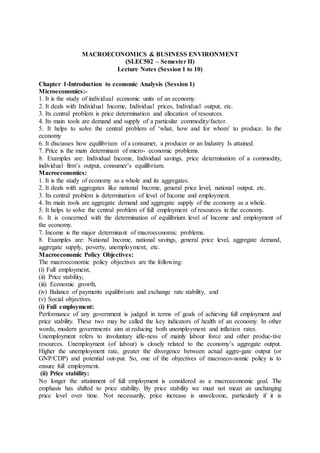
  • 38. 38 Classical Aggregate Supply Model To arrive at the Classical Aggregate Supply Model, we need to look at the production function and thereby the demand and supply functions for labor. Production Function As studied in Managerial Economics, the Production function gives us the relationship between the factor inputs and the output. What holds true about a firm holds true for the economy as well, the Real Output produced is a function of the land, labor, capital and enterprise. Other things remaining constant in the short run, the production is a function of the capital stock of the economy and the labor force. Y = f(K, N) Y = Real GDP K = Capital Stock N = Labor Employed In the short run, the capital stock and technology is assumed to be constant and hence the output produced would be a function of the labor employed. Y = f(N) The output increases as represented on the Y axis with an increase in the employment of labor on the X axis but a diminishing rate as shown in the diagram below: Source: Google Images
  • 39. 39 Demand for Labor Assuming that there is pure competition the demand for labor would reflect its marginal productivity and firms would keep on hiring till the value of the marginal product is greater than the money wage rate W = P * MPL W = Money wage rate P = Price Level MPL = Marginal Productivity of Labor Diving both the sides of the equation by the price level, we get W/P = MPL Which implies that the real wage in the economy would be a reflection of the marginal product of labor which is diminishing as more and more labor is employed. Source: ICFAI Center for Management Research
  • 40. 40 As seen in the above diagram, at a higher real wage rate the firms are only willing to employ labor to a point where the marginal product is high and thereby employ lesser workers at a high real wage and vice-versa. Supply Function of Labor The supply of labor is directly proportionate to the real wages and hence its an upward sloping curve. Ns = f(W/P) Ns = Supply of Labor W/P = Real Wage Rate Source: ICFAI Center for Management Research Deriving the Aggregate Supply Curve As per the Say’s Law, the supply create its own demand and the Output Y is determined by the labor market. In the first portion of the diagram below, the demand and supply curve lead to an employment of N at a real wage rate of (W/P), when we go down to the second portion of the diagram, we see that with this labor employed of N in the Production Function which
  • 41. 41 reflects the diminishing returns and we arrive at an equilibrium output of Y and this would adjust to a rise in the real wage rate giving us a perfectly inelastic aggregate supply curve in the third portion of the diagram. Source: ICFAI Center for Management Research
  • 42. 42 Keynesian View of the Aggregate Supply Model The Classical approach to Aggregate Supply was based on the fact that the labor market is completely flexible and the money wages would easily move up or down and the unemployment existing in the economy is voluntary in nature. However, this didn’t happen during the Great Depression where we had large scale unemployment and an involuntary one and thereby John Maynard Keynes came with his view of the Aggregate Supply Model where he said that the money wages are sticky and the labor market is not that flexible to respond to the unemployment. Hence as per Keynes the Aggregate Supply Curve is a J shaped with three distinct segments, the first flat segment shows the inflexibility of labor market and output can be expanded without an increase in the price level, the second segment or the curvy segment shows the flexibility in the labor market where output could be expanded at a higher price level and the last segment is the vertical segment which indicates that the output has reached the full employment level and cannot be expanded and any attempt to expand output would just result in higher price levels. This J shaped Aggregate Supply curve is illustrated in the upcoming chapters.
  • 43. 43 Inflation: Inflation is defined as a continuous increase in the aggregate price level of the economy. The aggregate price level is measured as a weighted average of prices in the economy. There are two primary indices to measure the aggregate price level. The index that tracks the change in retail prices of essential goods and services consumed by households is the Consumer Price Index or CPI. The Whole sale price index or WPI is a weighted average of the price of a representative basket of wholesale goods purchased by the producers and businessmen. So WPI does not include services, whereas the retail price index does. While CPI is the most relevant index for the consumer as it shows the increase in their spending, it is not a fully accurate cost of living indicator since it does not included all goods and focuses on certain goods and services more than others. The weightage of food in the CPI is close to 50%, but most households don’t spend nearly that much of their overall expenditure on food. For many consumers, major part of expenditure is on services such as education, health care and transportation, where inflation levels are much higher. In India, the CPI is used as an indicator of inflation. The rate of inflation is expressed as a percentage. The formula is Rate of inflation = {Price level (year t) – Price level (year t-1)} *100 Price level (year t-1) According to the National Statistical Office retail inflation accelerated to 6.93% in July 2020 from 6.23% in the preceding month, with food inflation rising to 9.62% in July 2020 from the June level of 8.72%. Inflation can be classified as: According to Degree: a. Creeping or crawling Inflation (< 2%) b. walking inflation (<5%) c. Running Inflation (<10%) d. Galloping Inflation (<25%) e. Hyperinflation (>25%)
  • 44. 44 While creeping inflation is a very low rate of inflation, with a slight pressure on prices, Galloping inflation and hyper- inflation is a situation where the prices of goods and services rise uncontrollably over a time period as was seen in Zimbabwe Disinflation is a situation where the rate of inflation falls – it is a slowdown in the rate of increase of the general price level of goods and services Deflation is a situation of falling prices. According to causes: Demand Pull Inflation takes place when aggregate demand increases faster than the economy’s ability to produce those goods and services. The causes of demand pull inflation can be a) Increase in Consumption and Investment will cause aggregate demand to increase b) Exchange rate: A depreciation of exchange rates can increase exports and thus lead to increase in aggregate demand c) Higher fiscal spending due to a stimulus d) Expectations: Sometimes simply the expectation of inflation can itself lead to higher actual prices as all wage, rent contracts are revised upwards to take care of the higher expected inflation. An increase in aggregate demand is shown by the rightward shift of the Aggregate Demand Curve. In the following diagram, the AD curve has shifted right from AD0 to AD1 leading to an increase in aggregate prices from P0 to P1. It can be observed that this price increase has been accompanied by an increase in national output as well. Any Demand Management policy – Fiscal, Monetary or Trade shifts the AD curve rightwards and causes inflation to take place. In fact a big dilemma of policy making is that there is a tradeoff between growth and inflation. Fig 1: Demand Pull Inflation
  • 45. 45 Source : www.economicshelp.org Cost Push Inflation: takes place when the Aggregate Supply curve shifts upwards primarily due to an increase in the cost of production. The main causes of supply side inflation are as follows a) Supply shock: It can be a result of a sudden rise in the prices of essential commodities. An increase in price of crude oil declared by OPEC can be an example as oil is a necessary raw material across sectors. b) Higher wages: When wages are increased maybe due to active trade unions, companies pass on the higher cost to higher retail prices. c) Imported inflation: Increase in prices of imported raw materials can also increase the retail prices of finished products. d) Higher taxes: Hike in indirect taxes like GST, sales tax and excise duties can also lead to cost push inflation as the AS curve will inflation by forcing prices up. In the following diagram, the AS curve has shifted upwards, leading to an increase in prices. A difference here is that this increase in prices is not accompanied by an increase in output. The
  • 46. 46 leftward shift of AS curve from AS0 to AS1 leads to an increase in prices from P0 to P1. The output shrinks from Y0 to Y1. Fig 2: Cost Push Inflation Source : www.economicshelp.org Cost Push inflation is also called supply side inflation. Wage Price Spiral: Combination of both demand pull and cost push can be a result of indexation of wages when the workers demand higher wages due to increasing retail prices. In this case a demand full inflation results in higher prices leading to higher wages and a higher inflation. Costs of Inflation: a) Redistribution of income and wealth- borrowers’ gain and creditors lose. All those who earn fixed income such as those who rely on pensions and interest lose whenever inflation takes place Balance of payments effect- exports become expensive. Hence exchange rate depreciates. b) Uncertainty about the value of money may lead to a flight of capital to other economies as people would want to protect the real value of their money. c) Exports become more expensive due to inflationary price rise. Consumers are also tempted to import goods from abroad. On both counts, the current account deficit worsens. d) There is a “menu cost “of changing all price tags without any real gin to the economy
  • 47. 47 e) Inflation is an indicator of health of an economy and high levels of inflation reduces the credibility of the country and may impact foreign and domestic investment leading to a slowdown in growth. Inflation Targeting: When the Central Bank of the economy sets a target level of inflation, it is called inflation Targeting”. In India, RBI has a target of keeping inflation at 4% with a tolerance limit of 2%. This meant that inflation should be between 2% and 6% and any deviation from this range is outside the comfort level of RBI and monetary policies are initiated to get the inflation rate within that range. It is desirable that the economy faces a slight pressure on price to keep the producers motivated and hence a creeping to walking inflation is a healthy sign for the economy. Stagflation: Stagflation is a situation of a simultaneous increase in inflation and stagnation of economic growth. This situation was first recognized during the 1970's, where it was seen that in high unemployment coexisted with high inflation. One reason cited for this was oil price shocks. Stagflation cannot be explained by the earlier discussion of demand pull inflation as it was seen in the diagram that the higher rates of inflation were always accompanied by higher growth and lower unemployment. This led to the famous model of the Philips curve which using empirical data described this trade- off between inflation and unemployment Origin of Phillips Curve An article titled “The Relationship between Unemployment and the Rate of Change of Money Wages in the United Kingdom, 1861-1957” by A. W. Phillips was published in 1958. The article out forth a negative correlation between the rate of unemployment and the rate of inflation. The data showed that the years when unemployment rate was high, inflation was low and the years with low unemployment experienced high inflation. Here, A. W. Phillips put forth that the Phillips curve is an inverse relation between rate of unemployment and rate of increase in money wages. The higher the unemployment, the lower the
  • 48. 48 rate of wage inflation. In other words, the trade-off is between wage inflation and unemployment: gw = -a (u – u*) where gw is the growth rate in wages u is the actual unemployment u* is the natural rate of unemployment a is the responsiveness of wages to unemployment The equation shows that wages are falling when u > u*. Similar relation was also found by Paul Samuelson and Robert Solow in the U.S. economy, reporting a negative correlation between inflation and unemployment in the United States also. This relation was found in other economies as well and came to be known as the Phillips Curve. The Phillips Curve The Phillips Curve is the graphical depiction of the short-term relationship between unemployment and inflation in an economy. The curve is a downward sloping curve representing the negative, or inverse, relationship between the unemployment rate and the inflation rate in an economy. The relation can be explained using Keynesian economics that propounds the use of monetary and fiscal policy to bring growth by increase in aggregate demand. This stimulus is expected to increase employment and output accompanied by increasing price level. In order to ensure price stability, policymakers need to reduce output and employment in the short run.
  • 49. 49 Figure 3: Source: Lumen Learning Samuelson and Solow stated that the Phillips Curve could be used by policymakers by selecting the unemployment – inflation combination as preferred by the economy. To illustrate, point A in Fig 3, depicts a situation of high unemployment and low inflation. Policymakers would endeavour to increase output by possibly increasing government spending and/ or cutting taxes to push demand in the economy (Fig.3). Given the implementation of expansionary fiscal policy, employment and output are expected to rise. However, as there is a limit to how much the output can be increased given inelastic aggregate supply curve, once reached, any further increase in demand leads to inflation. This position is explained by point B. Also, at point B, the economy experiences low unemployment but high inflation. Although, policymakers would prefer both unemployment and low inflation to be are low simultaneously, it appears to be nearly impossible based on historical data studied by Phillips, Samuelson, and Solow.
  • 50. 50 Figure 4 Phillips Curve Source: Lumen Learning Long-run Phillips Curve American economist and chief proponent of monetarism, Milton Freidman, put forth that the monetary policy is unable to reduce unemployment by raising inflation, in paper titled “The Role of Monetary Policy.” in 1968. His belief was primarily based by the classical macroeconomic theory that money being a nominal variable, cannot have an impact on a real variable such as unemployment or output. Further, in 1970, another Nobel Prize-winning economist, Edmund Phelps, stated that there is no long-term trade-off between inflation and unemployment. Both the economists together gave us the ‘Friedman-Phelps Phillips Curve’ that depicts the long- term relationship between the inflation rate and the unemployment rate in an economy. It is vertical (Fig.5), representing the inelastic nature of unemployment to price levels in an economy. The ‘Friedman-Phelps Phillips Curve’ settles at the natural rate of unemployment.
  • 51. 51 Figure 5 Source: Lumen Learning (gw - πe) = -a (u – u*) Where πe is the level of expected inflation. The above equation shows that as long as there is excess wage inflation over expected inflation, actual unemployment will be lower than natural rate of unemployment (Point B). This also means that policy efforts to reduce unemployment will result in temporary adjustments along the short-run Phillips curve. However, unemployment will revert to the natural rate of unemployment and will result in higher inflation. Let’s assume the economy is at point A (Fig. 5) at an initial level of unemployment and inflation rate. In case the government implements an expansionary policy to reduce unemployment further, then inflation will increase as aggregate demand shifts to the right. This causes movement along the short-run Phillips curve, to point B, where unemployment has fallen and inflation has increased. However, this is an unstable equilibrium. The increased aggregate demand, on account of expansionary fiscal policy, makes producers employ more workers to meet demand, thereby reducing unemployment. However, the higher inflation fuels workers’ expectations of future inflation changes. This expectation causes a shift in the short-run Phillips curve to the right, thereby moving from an unstable equilibrium point B to the stable equilibrium
  • 52. 52 point C. But at point C, the unemployment rate has reverted to its natural rate, but inflation remains higher than its initial level. Hence policy makers can try to reduce the Natural Rate of Unemployment, the unemployment rate towards which the economy moves in the long term. It is evident from the above equation that the tradeoff between growth and inflation can be explained by the short run Philips curve and it is only the expectations augmented Philips curve which can justify the possibility of stagflation in the economy. ---------------------------------------------------------------------------------------------------------------------
  • 53. 53 Demand for Money and Determination of Interest Rate Definition of Money Money is a unit of exchange and has evolved to solve the problem of the barter system. Money can buy all goods and services, and this is more convenient than goods buying goods. “Money buys goods and goods buy money, but goods do not buy goods” (Robert W). Functions of Money : Money performs four functions: A medium, a unit, standard, and a store 1. Medium of Exchange: Money is a fungible mode of exchange for goods and services, it is a marked improvement from the barter system and an efficient way of transacting in a complex economy. Its birth has improved exchange for all parties. 2. Unit of Account: For money to serve as medium of exchange, it must have a common denominator for measuring goods and service. Everything that we purchase with money is measured in different units (gm, litres, yarns, inches). There is a need for a common yardstick to measuring value of different goods and service. Money provides that singular unit of account and helps to measure all goods and services in a common denomination - rupees, pounds, dollars. All goods and service thus have a single measure of value. The prices of all goods and services can be fixed in terms of money. Money gives a monetary unit of measure to all goods and services, and hence a relative comparison of different values of different goods and services is facilitated. Knowing the value or price of a good in terms of money, enables both the supplier and the purchaser of the good to make decisions about how much of the good to supply and how much of the good to purchase. 3. Store of Value: For money to retain its purchasing power or to ensure it can be used in future, it needs to have a store of value. Money should be stored easily to serve as a medium of exchange and command a purchasing power at a future date too. Hence money holds its value in future time. Of course, inflation, and deflation render a compromise in purchasing power of money, Yet it remains valuable as a medium of exchange in future times, as it is not perishable and is readily accepted everywhere.
  • 54. 54 4. Standard of deferred Payment: In an economy everything is not instantaneously cash settled. Buyers can buy goods and services in the present and can pay for them in future. In other words, the payments are deferred, and can be made in future. Money has made this function easier as loans can also be taken and settled in future. Money can be used as a standard benchmark for specifying future payments for current purchases, that is, buying now and paying later. The Demand for Money : Classical Versus Keynesian Theories The demand for money is the demand for real balances. A stable demand for money is a cornerstone of monetary policy, and hence it needs to be subjected to extensive examination and scrutiny. With passage of time, theories of Money demand have evolved. The theories explore demand for money and their determinants. This section touches on two fundamental approaches to money supply - The Classical, and the Keynesian approach. Classical Approach to demand for Money : The classical demand for money hinges on assumption of neutrality of money. Money serves as a medium of exchange and changes in money supply affect absolute prices and not relative prices. There are two version to the Classical School: a) Cash Transaction Approach / Fisher Quantity theory of Money, and b) Cash Balance Approach / Cambridge School Cash Transaction Approach: Popularly known as the Quantity theory of Money, this was postulated by Irwing Fisher in his famous book: “Purchasing Power of Money”. It analyses the relation between quantity of money and Price level. The famous Fishers equation is given by: Where M = Money Supply, V = Velocity of Circulation, P = Price Level, and T = Transactions in an economy (quantity of goods and services offered in an economy). Holding T and V constant, we can see that increases in the money supply will cause price levels to increase. In other words, this equation means that in an economy, the total value of all goods sold during any period (PT) is equal to
  • 55. 55 the total quantity of money spent during that period (MV). In other words, the price levels are directly proportional to the quantity of money in circulation in the economy. So, if the supply of money is doubled, then the price of money would double too. Fisher stresses that money is fundamentally a medium of exchange and people demand money to fulfil their need for transactions. However, money also fulfils future needs and needs to be stored. Another group of economists belonging to the Cambridge School - economists Marshal, Pigou, Robertson etc. opined that “The amount of money which is kept by the individual, commercial institutions and government to meet their day to day needs is called demand of money”. The value of money is determined by cash balances that people demand, and they evolved a separate set of equations called the cash balance equations. Cambridge Version where M = Money demand, P = Price Level, Y = Real Income, K = the portion of real income which people want to keep with them in the form of cash. This version stressed that people like to hold money in form of cash. It is K that determines demand for money and makes demand for money a positive function of real national income. If national income increases people demand for money will also increase, by the coefficient K. If K= 0.1, and National income is Rs. 100 crores, the economy demand for cash balances is Rs. 10 crores. Both Fisher and Cambridge opined that money demand is a positive function of National income or GDP. However, Fisher concentrated on the medium of exchange function, whereas Cambridge stressed on the Store value function. Both the versions had a fatal flaw, in that they could not explain role of interest rate as a determinant to demand for money. Keynes Demand for Money : Keynes brought a paradigm change in the theory of demand for money by specifying the role of interest, which was ignored by his predecessors. He divided the demand for money into three motives - Transactionary Motive ( b), a Precautionary Motive ( c), and a Speculative Motive .
  • 56. 56 Transactionary Motive: People demand cash to meet their transactions, and to meet their payments. This part of demand is a positive function of Income and is inextricably linked with medium of exchange in a money-exchange economy. Precautionary Motive: Money is demanded by people to meet their contingency requirements. Both demand for transaction and precautionary motive are determined by income and are vaguely analogous to what the classicals opined. The Speculative Demand for Money: The cornerstone of Keynesian analyses is speculative demand for money or demand for idle cash balances, and this brings in a paradigm change. Keynes opined that money merely is not just a medium of exchange but is an asset which competes with other assets like bonds in the Portfolio of every investor. The wealth of an individual has idle cash and Bonds. Individuals after meeting their precautionary and transaction demands, use money as an asset. He made a simplistic assumption that there are Bonds and idle Cash only in every investor’s portfolio. Bonds earn an interest rate, whereas idle Cash does not. But Bond prices fluctuate, and income can be more than wiped out if bond prices fall in future. Keynes believed that interest rate expectations of all investors or portfolio holders vary, but at very high rate of interest all asset holders would want to convert their idle cash into bonds. Hence, the demand for idle cash balances, known as speculative demand, will be very low. Similarly, if rate of interest is very low, people would not want to invest in bonds and keep more idle cash. At low rates of interest, the bond prices are high (Bond prices and rate of interest are inversely related)i. So, speculative demand for money is very high. Hence at high rate of interest people have low demand for Idle cash balances and at low interest rates people demand for idle cash balances increase. Speculative demand for Money Fig: 1 Interest