Lecture Notes

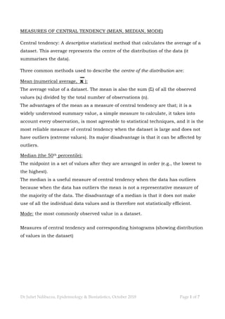
1. Dr Juliet Ndibazza, Epidemiology & Biostatistics, October 2018 Page 1 of 7
MEASURES OF CENTRAL TENDENCY (MEAN, MEDIAN, MODE)
Central tendency: A descriptive statistical method that calculates the average of a
dataset. This average represents the centre of the distribution of the data (it
summarises the data).
Three common methods used to describe the centre of the distribution are:
Mean (numerical average, x ):
The average value of a dataset. The mean is also the sum (Σ) of all the observed
values (xi) divided by the total number of observations (n).
The advantages of the mean as a measure of central tendency are that; it is a
widely understood summary value, a simple measure to calculate, it takes into
account every observation, is most agreeable to statistical techniques, and it is the
most reliable measure of central tendency when the dataset is large and does not
have outliers (extreme values). Its major disadvantage is that it can be affected by
outliers.
Median (the 50th percentile):
The midpoint in a set of values after they are arranged in order (e.g., the lowest to
the highest).
The median is a useful measure of central tendency when the data has outliers
because when the data has outliers the mean is not a representative measure of
the majority of the data. The disadvantage of a median is that it does not make
use of all the individual data values and is therefore not statistically efficient.
Mode: the most commonly observed value in a dataset.
Measures of central tendency and corresponding histograms (showing distribution
of values in the dataset)

2. Dr Juliet Ndibazza, Epidemiology & Biostatistics, October 2018 Page 2 of 7
✓ If the mean and the median are approximately equal the distribution of the
values around the mean is symmetric, and the histogram is bell-shaped
(normal or symmetric distribution).
✓ If the mean is greater than the median (e.g. due to high outliers), the histogram
is right skewed.
✓ If the mean is less than the median (e.g. due to low outliers), the histogram is
left skewed.
NB: Even though we can always determine both the mean and median, we must
determine which measure is more appropriate to use when there is a large
difference between the mean and median.
Generally, when the data is skewed, the median is more appropriate to use as the
measure of central tendency. We generally use the mean as the measure of central
tendency when the data is fairly symmetric. It is often important to be given both
measures of central tendency; the difference between the mean and median is
important since the direction and magnitude of that difference helps us envision
the likely shape of the histogram.
Using excel dataset: Mother age and height – symmetric and skewed
1. Calculate the mean, median and mode for the mothers’ (a) age (b) heights.
2. Group the data, and plot a graph (in excel) to show the distribution of the
mothers’ (a) age (b) heights.
3. Is your histogram symmetric, right skewed or left skewed?

3. Dr Juliet Ndibazza, Epidemiology & Biostatistics, October 2018 Page 3 of 7
MEASURES OF DISPERSION (RANGE, VARIANCE, STANDARD DEVIATION)
It is also useful to have an idea of how the values spread out around the central
value. i.e. how far apart are the individual observations from a central value for a
given variable? The measures of dispersion show how far the values differ from the
mean, or how similar a set of values are to each other.
Range: the interval between the largest and the smallest values. It is the simplest
measure of dispersion, but is based on only two observations and gives no idea of
how the observations are arranged between the largest and the smallest values.
Percentile: the percentile represents the percentage of the values that lie below a
specified observation. For example, the median is also known as the 50th
percentile because half of the data or 50% of the observations lie below the
median. The median is also known as the Second quartile (Q2)
Lower quartile (First quartile (Q1)): 25% of the observations lie below this
percentile.
Upper quartile (Third quartile (Q3)): 75% of the observations lie below this
percentile.
Inter-quartile range (IQR): the difference between the upper and the lower quartile.
The interquartile range represents the middle 50% of the values in the dataset.
What is the proportion of the mothers that have a height greater than 165cm?
Standard deviation: This is the average distance that each observation is from the
mean. If the values within a dataset are not very different from one another, the

4. Dr Juliet Ndibazza, Epidemiology & Biostatistics, October 2018 Page 4 of 7
standard deviations will be small & the values will be grouped closely around the
mean. If the values within a dataset vary considerably, the standard deviations
will be large & the values will be scattered widely around the mean.
As a rule of thumb about 2/3 of the data fall within one standard deviation of the
mean.
The standard deviation is calculated using every observation in the data set, and
because it is influenced by outliers, it is a sensitive measure.
4. Which graph has a larger standard deviation (the upper or the lower) and why?
Calculating the standard deviation
If the weights (kg) for ten MPH students were:
44, 34, 54, 33, 64, 42, 48, 56, 45, 68
The total number of observations (n) = 10
Each observation is represented by (x)
The mean ( x ) = 48.8
The deviation from the mean for each observation = (x – x)
The square of the deviation from the mean for each observation = (x – x)2

5. Dr Juliet Ndibazza, Epidemiology & Biostatistics, October 2018 Page 5 of 7
Weight (x) (x – x) (x – x)2
44 (44 – 48.8) = - 4.8 (-4.8 X -4.8) = 23.0
34 -14.8 219.0
54 5.2 27.0
33 -15.8 249.7
64 15.2 231.0
42 -6.8 46.2
48 -0.8 0.6
56 7.2 51.8
45 -3.8 14.4
68 19.2 368.6
The sum of the squares of the deviation from the mean for all observations
= Σ(x – x)2
= (23.0 + 219.0 + 27.0 + 249.7 + 231.0 + 46.2 + 0.6 + 51.8 + 14.4 + 368.6) =
1,231.3
The variance = Σ (x – x)2/ n – 1
The standard deviation = √ Σ (x – x)2/ n – 1 = √(1231.3/9) = √(136.8) = 11.7
NB: The standard deviation is the square root of the variance
Why are the standard deviation and the mean important?
The normal distribution (bell-shaped curve, see graph below) is the histogram we
obtain when the distribution of the values of a dataset is symmetrical around the
mean. The shape of any distribution is determined by the mean, and the standard
deviation. The highest point on the curve is the mean.

6. Dr Juliet Ndibazza, Epidemiology & Biostatistics, October 2018 Page 6 of 7
x-3s x-2s x-1s x x+1s x+2s x+3s
When you plot the weights for all the MPH students, with a mean (x) weight of
48.8kg and a standard deviation (s.d) of 11.7:
68% of the weights for this class will lie between 1 standard deviation (s.d) of the
mean. i.e between (x-1s) and (x+1s). That is to say, 68% of the weights for this
class will lie between between (48.8 – 11.7) and (48.8 + 11.7).
That is to say, 68% of the weights for the class will lie between 37.1kg and 60.5kg.
Meanwhile, 95% of the weights for the class will lie between 2 standard deviations
of the mean.
That is to say, 95% of the weights for the class will lie between (x-2s) and (x+2s)
Or that, 95% of the weights for the class will lie between (48.8 – 23.4) and (48.8 +
23.4). The same as saying, 95% of the weights for the class will lie between 25.4kg
and 72.2kg.
And 99% of the weights for the class will lie between 3 standard deviations of the
mean.
That is to say, 95% of the weights for the class will lie between (x-3s) and (x+3s)

7. Dr Juliet Ndibazza, Epidemiology & Biostatistics, October 2018 Page 7 of 7
Or that, 95% of the weights for the class will lie between (48.8 – 35.1) and (48.8 +
35.1). The same as saying, 95% of the weights for the class will lie between 13.7kg
and 83.9kg.
5. Now calculate the standard deviation for the mothers’ heights.
6. Obtain the range that will contain 68% of the mother’s heights.
7. Obtain the range that will contain 95% of the mother’s heights.