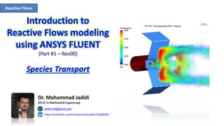
Introduction to Reactive Flows modeling using ANSYS FLUENT (Part #1 – Rev00) Species Transport

1. Reactive Flows
https://ir.linkedin.com/in/moammad-jadidi-03ab8399
Jadidi.cfd@gmail.com
Dr. Mohammad Jadidi
(Ph.D. in Mechanical Engineering)

2. Presented by: Mohammad Jadidi 2
Equations governing reacting flowsReactive Flows
FLUENT can model the mixing
and transport of chemical species
by solving conservation equations
describing convection, diffusion,
and reaction sources for each
component species.
 Conservation equations
– Continuity equation (conservation of mass)
– Transport of momentum
– Transport of Energy
– Transport of molecular species
 Equation of State
 Turbulence Transport
– Transport of turbulent kinetic energy
– Transport of turbulent dissipation rate
– Transport of turbulent Reynolds stresses
– Transport of moments such as 𝑢′
𝑖 𝑌′
𝑖

3. Presented by: Mohammad Jadidi 3
Relevant quantitiesReactive Flows
 Mole fraction (𝑋𝑖)
 Fraction of total number of moles of a given species in a mixture
 Mass fraction ( 𝑌𝑖)
 Fraction of mass of a given species in a mixture
 Relation between
 Mixture molecular weight 𝑀 𝑤,𝑚𝑖𝑥 = ෍
𝑖
𝑋𝑖 𝑀 𝑤,𝑖 = ෎
𝑖
𝑌𝑖
𝑀 𝑤,𝑖
−1
𝑌𝑖 = 𝑋𝑖
𝑀 𝑤,𝑖
𝑀 𝑤,𝑚𝑖𝑥
𝑌𝑖=
𝑚 𝑖
𝑚 𝑇𝑜𝑡
𝑋𝑖 =
𝑁𝑖
𝑁 𝑇𝑜𝑡

4. Presented by: Mohammad Jadidi 4
Species Transport EquationsReactive Flows
To solve conservation equations for chemical species, ANSYS Fluent predicts the
local mass fraction of each species, 𝑌𝑖 , through the solution of a convection-
diffusion equation for the 𝑖 𝑡ℎ species
 𝑅𝑖 is the net rate of production of
species by chemical reaction (described in
details in next presentation)
 𝑆𝑖 is the rate of creation by addition from
the dispersed phase plus any user-defined
sources
 An equation of this form will be solved for N-1 species where N is
the total number of fluid phase chemical species present in the
system.
 Since the mass fraction of the species must sum to unity, the 𝑁 𝑡ℎ
mass fraction is determined as one minus the sum of the N-1
solved mass fractions.
 To minimize numerical error, the 𝑁 𝑡ℎ
species should be selected as
that species with the overall largest mass fraction, such as 𝑁2when
the oxidizer is air
Note:

5. Presented by: Mohammad Jadidi 5
Mass Diffusion in Laminar FlowsReactive Flows
Ԧ𝐽𝑖 is the diffusion flux of species ,which arises due to gradients of
concentration and temperature.
Ԧ𝐽𝑖 = −𝜌𝐷𝑖,𝑚 𝛻𝑌𝑖 − 𝐷 𝑇,𝑖
𝛻𝑇
𝑇By default, ANSYS Fluent uses the
dilute approximation (also called
Fick’s law) to model mass
diffusion due to concentration
gradients
𝐷𝑖,𝑚: mass diffusion coefficient for species in the
mixture.
𝐷 𝑇,𝑖: thermal (Soret) diffusion coefficient.
Note:

6. Presented by: Mohammad Jadidi 6
Mass Diffusion in Laminar Flows-Dilute approximation (also called Fick’s law)Reactive Flows
Ԧ𝐽𝑖 = −𝜌𝐷𝑖,𝑚 𝛻𝑌𝑖
𝐷𝑖,𝑚: mass diffusion coefficient for species in the mixture.
Modeling of diffusion
velocities by Fick-like
expression
𝐿𝑒𝑖 =
𝑘
𝜌𝐶 𝑝 𝐷𝑖,𝑚
𝑘 : thermal conductivity.
𝑈𝑖 𝑌𝑖 = −𝐷𝑖,𝑚 𝛻𝑌𝑖=−𝐷𝑖,𝑚
𝜕𝑌 𝑖
𝜕𝑥 𝑖
Species diffusion fluxes
𝜌𝑈𝑖 𝑌𝑖=-
𝑘
𝐿𝑒𝑖
𝜕𝑌 𝑖
𝜕𝑥 𝑖
Lewis number

7. Presented by: Mohammad Jadidi 7
Mass Diffusion in Laminar Flows-Maxwell-Stefan equationsReactive Flows
For certain laminar flows, the dilute
approximation may not be
acceptable, and full multicomponent
diffusion is required. In such cases,
the Maxwell-Stefan equations can
be solved

8. Presented by: Mohammad Jadidi 8
Mass Diffusion in Turbulent FlowsReactive Flows
In turbulent flows Ԧ𝐽𝑖 = (−𝜌𝐷𝑖,𝑚 +
𝜇 𝑡
𝑆𝑐𝑡
)𝛻𝑌𝑖 − 𝐷 𝑇,𝑖
𝛻𝑇
𝑇
𝑆𝑐𝑡=
𝜇 𝑡
𝜌𝐷𝑡
: turbulent Schmidt number
𝜇 𝑡 : turbulent viscosity
𝐷𝑡 : turbulent diffusivity
The default
𝑺𝒄 𝒕 is 0.7

9. Presented by: Mohammad Jadidi 9
Treatment of Species Transport in the Energy EquationReactive Flows
෍
𝑖=1
𝑛
ℎ𝑖 𝐽𝑖
𝐿𝑒𝑖 =
𝑘
𝜌𝐶 𝑝 𝐷𝑖,𝑚
transport of enthalpy due to species diffusion
transport of enthalpy due to species
diffusion can have a significant effect on
the enthalpy field and should not be
neglected. In particular, when the Lewis
number for any species is far from unity,
neglecting this term can lead to
significant errors.
𝑘 : thermal conductivity.
Note:

10. 10
This tutorial demonstrates the use of
species transport model in ANSYS
FLUENT to study the species
diffusion and mixing characteristics
in baffled reactors
Presented by: Mohammad Jadidi
Species Transport tutorial #1Reactive Flows
10

11. Presented by: Mohammad Jadidi 11
Reactive Flows Species Transport tutorial #2
Test Case
A propane jet issues into a co-axial stream
of air. There is turbulent mixing between
the species in the axisymmetric tunnel.
Only half of the domain is considered due
to axial symmetry.
Material Properties Geometry Boundary Conditions
Density: Incompressible ideal
gas law
Viscosity: 1.72X10
–5
kg/m-s
Tunnel length = 2 m
Tunnel diameter = 0.3 m
Propane jet tube:
Inner diameter = 5.2 mm
Outer diameter = 11 mm
Inlet velocity of air = 9.2 m/s
Inlet velocity of Propane – Specified as
fully developed profile
Inlet temperature (both streams) =
300 K
Temperature at the wall = 300 K
http://www.sandia.gov/TNF/DataArch/ProJet.html

12. 12
Multiphase Flows
Thanks
https://ir.linkedin.com/in/moammad-jadidi-03ab8399
Jadidi.cfd@gmail.com
Dr. Mohammad Jadidi
(Ph.D. in Mechanical Engineering)
End of part #1 Next part: