SlideShare ist ein Scribd-Unternehmen logo
1 von 33
8/19/2022 Berhanu G(Dr) 1
Line and Surface Integrals
4. 1 Line Integral
C
A
B
• Let C be a smooth space curve with initial
point A and terminal point B, parameterized by
its arc length s:
• And let f( x, y, z) is a scalar field defined at each point on C.
• The line (curve) integral of f along C from A to B, w.r.t. arc length s,
is defined by
r (s) = x(s)i + y(s) j + z(s) k, asb
(so that r(a)=A and r(b)=B )
( , , ) ( ), ( ), ( )
( )
C
b
a
f x y z ds f x s y s z s ds

 
• If C is closed, the line integral is denoted by
C
fds

8/19/2022 Berhanu G(Dr) 2
• Example 1: Integrate f(x,y)=xy2 over a circular
arc given by
r (s) = cos(s) i + sin(s) j , 0 s  /2
• Remark: If a curve C is parameterized by any parameter, say, t :
2 2
/ 2
0
2
cos( )sin ( )
3
C
xy ds s s ds

 
 
C
• Solution: On C, x =cos(s) ; y= sin(s)
 f(x,y)=xy2 =cos(s). sin2(s) , on C.
Therefore,
r (t) = x(t)i + y(t) j + z(t) k, a  t  b,
'( )
ds
ds dt t dt
dt
  r
then, making change of variable:
we get,
( , , ) ( ( )) '( )
C
b
a
f x y z ds f t t dt

  r r
8/19/2022 Berhanu G(Dr) 3
• Example 2: Evaluate ( 4 )
C
xy z ds


• Solution: C is given by
r (t) = A + t (BA) , 0  t  1
= 2t i + t j + (1+2t) k, 0  t  1.
So, on C, xy +4z = (2t)t + 4(1+2t) = 2t2 + 8t + 4
and, ds = |r(t) | dt . But |r(t) |= | 2i + j + 2 k | = 3
 ds = 3dt
Therefore,
when C is a straight line segment from point A(0,0, 1) to B = (2, 1,3).
8/19/2022 Berhanu G(Dr) 4
Usually, line integrals that involves a vector field F( x, y, z) that defined
on C has the following form:
C
r(t)
A
B
• Or, representing C by
r (t) = x(t)i + y(t) j + z(t) k, a  t  b,
.
C
d
 F r
where, F( x, y, z) = f1(x,y,z)i + f2 (x,y,z)j + f3 (x,y,z) k,
and, dr = dx i + dy j + dz k
( line integral of tangential
component of F )
That is,
1 2 3
( , , ) ( , , ) ( , , )
.
C
C
d f x y z dx f x y z dy f x y z dz
  
 
F r
'( )
d
d dt t dt
dt
 
r
r r ( , , ) ( ( ))
x y z t

F F r
Moreover, on C,
We get,
( ( )) '( )
. .
b
C
a
d t t dt

 
F r F r r
8/19/2022 Berhanu G(Dr) 5
• Example 3: Let F(x,y) = (x + y) i + (xy) j . Evaluate
when C is: (a) the parabola y=x2 from (1,1) to (4,2)
(b) the circle x2+y2 = 1
• Solution: (a) F.dr = (x+y)dx + (xy)dy. But on C, y=x2 , dy=2xdx
= (x+x2) dx + (xx2)2x dx
= (x + 3x2 2x3) dx, 1  x  4.
Hence,
(b) C, parametrically, r (t) = cost i + sint j , 0  t  2
r (t) = cost i + sint j ,  r (t) = sint i + cost j ,
and, F(r(t) ) = (cost + sint) i + (costsint) j .
Hence,
.
C
d
 F r
( ) ( )
.
C C
d x y dx x y dy
   
 
F r
4
2 3
1
34
3
( 3 2 )
x x x dx
   

2 2
0 0
( ( )) '( ) (cos(2 ) sin(2 )) 0
. .
C
d t t dt t t dt
 
   
  
F r F r r
8/19/2022 Berhanu G(Dr) 6
• Exercise:
1) Let F(x,y) = x i + x2 j . Evaluate
Ans.  4
(1,0)
( 1,0)
.d

 F r
along curve C , from (1,0) to (1,0) in the xy-plane, given by
(a) the semi-circle of radius 1
(b) the polygonal path (line segments) shown in the figure below.
(1,0) (1,0)
(1,1)
(0,1)
2) Evaluate
where C is the circle x2+y2=4, oriented counterclockwise.
C
ydx xydy


Ans. (a) 0; (b) ½
8/19/2022 Berhanu G(Dr) 7
At each instant of time t, the particle may
be thought as moving in the direction of the
tangent to its trajectory, r(t).
Hence, F(r(t)).r(t) is the product of force
with a direction, and so has the dimension
of work. Therefore, the line integral
is the work done by the force F in moving the particle from A to B
over the path C.
( ( )) '( )
. .
b
C
a
d t t dt

 
F r F r r
Remark : Line integrals arise in many context. For example, consider
a force F causing a particle to move from point A to point B in space
along a smooth curve C whose vector equation r(t) is representing the
position of the particle at time t, such that atb,
C
r(t)
A
B
r (t)
8/19/2022 Berhanu G(Dr) 8
• Suppose C1 and C2 are different curves from point A to B, and
let F(x,y,z) be a vector space defined on both curves,
4. 2 Line Integral Independent of Path
A
B
C1
C2
• In a general case,
1
.
C
d
 F r and
2
.
C
d
 F r may not equal. (See, the above
exercise. )
• That means, the value of a line integral from point A to B may
depend on the curve (path) along which we integrate. (see, the
above exercise)
• However, for a particular F, if
for every curve C1 and C2 that join any point A to B , we say the
line integral of F is path independent.
1 2
. .
C C
d d

 
F r F r
• We will show that line integral of a conservative vector filed F is
path independent. Recall: F is conservative if F=f, for some
scalar field f (called potential of F)
8/19/2022 Berhanu G(Dr) 9
Theorem: (Fundamental Theorem of Line Integral)
Suppose C is a smooth curve from point A(x0,y0,z0) to B(x1,y1,z1) .
Let f (x,y,z) be a scalar field, continuously differentiable, on C.
Then,
A
B
C
Proof: Let r(t), for atb, represents C so that r(a)=A and r(b)=B.
( ) ( )
.
C
d f B f A
f  

 r
• Consequently, the line integral of f is path independent. Hence,
the line integral of f along every curve C from point A to B are
equal and can be written as
'( )
. ( ( ).
b
C a
d t dt
f f r t

 
 
r r
=
( ( ) ( ( )
b b
a
a
d
dt f t f t
  r r
( ( ) ( ( ) ( ) ( )
f b f a f B f A
   
r r
( ) ( )
.
B
A
d f B f A
f  

 r
8/19/2022 Berhanu G(Dr) 10
Theorem: (Line Integral of Conservative Vector Fields)
The line integral of a conservative vector field is independent of path.
In particular, if F is a conservative vector field and C is a curve from
point A to B, then
where  is a potential of F; i.e., F= 
Thus, the line integral of a conservative F over a curve C is the
difference of the values of its potential function at the end points of C.
( ) ( )
. .
C C
d d B A
 

  

 
r r
F
( ) ( )
.
C
d B A
 
 
 F r
Further, if C is a closed curve, then 0
.
C
d 
 F r
• The proof follows directly from the previous Theorem since,
8/19/2022 Berhanu G(Dr) 11
Example. Evaluate
2
(1, /8)
(0,0)
2 cos(2 ) 2 sin(2 )
x y dx x y dy



Solution: This is line integral of F(x,y) = 2xcos(2y) i – 2x2sin(2y) j
along certain curve from (0,0) to (1, /8). You can check that F is
conservative and its potential function is (x,y) = x2cos(2y). Hence,
along any curve in the xy-plane from (0,0) to (1, /8), we get
2
(1, /8)
8
(0,0)
2
2
2 cos(2 ) 2 sin(2 ) (1, ) (0,0)
x y dx x y dy


 
  


8/19/2022 Berhanu G(Dr) 12
Exercise.
2
(2,3)
(0,1)
(2 1) ( 1)
xy dx x dy
  

(a)
2. For the following integrals, C is the ellipse x2 + 4y2 = 16
(5,3,2)
(0,0,0)
.dr
 F
(b) , where F(x,y,z) = 3i + zj + (y+2z)k
1. Show that each of the following line integrals are independent
of path and evaluate the integrals.
.
C
dr
 F
(i) , F(x,y,z) = (2xy+z2)i + x2j + (2xz+  cos(z) )k
(ii)
2 3
C
3x ydx x dy


8/19/2022 Berhanu G(Dr) 13
• Green’s Theorem relates certain line integrals over a closed curve
with double integrals over plane region enclosed by the curve.
4. 3 Green’s Theorem
• Recall the following definition of double integrals:
If R ={ (x,y) | a  x b, g1(x) y g2(x) },
y=g1(x)
y=g2(x)
a b
R
 
2
1
( )
( )
R
( , )
( , )
g x
g x
b
a
f x y dxdy x y x
f y d
d
 
 
• OR, if R ={ (x,y) | h1(y) x h2(y) ,c y d },
 
2
1
( )
( )
R
( , )
( , )
h y
h y
d
c
f x y dxdy x y y
f x d
d
 
  c
d
R
8/19/2022 Berhanu G(Dr) 14
Theorem: ( Green’s Theorem)
2 1
1 2
R
( , ) ( , )
C
f f
f x y dx f x y dy dxdy
x y
 
 
  
 
 
 
 
Suppose C is a closed piecewise smooth curve in xy-plane oriented
counter clockwise, R is the region enclosed by C; and
F(x,y)= f1(x,y) i + f2(x,y) j . Then,
R
C
That is,
R
.
C
d dxdy
  
 
F r F.k
Note:
1. Observe the analogy between Fundamental theorem of Calculus,
Fundamental Theorem of line integrals, and Green’s Theorem.
2. Green’s Theorem can be used to evaluate line integrals over a
closed piecewise smooth curve in plane.
8/19/2022 Berhanu G(Dr) 15
Example: Use Green’s Theorem to evaluate
3
( ) ( 1)
C
x xy dx y dy
  

where C is the boundary of a square with vertices at the points
(1, 0), (2,0), (2, 1) and (1, 1), as shown in the figure below.
Solution: f1= x – xy and f2 = y3 +1 (1,0) (2,0)
(2,1)
(1,1)
R
C
3 2 1
R
( ) ( 1)
C
f f
x xy dx y dy dxdy
x y
 
 
    
 
 
 
 
2 2
1 1
1 1 1
0 0 0
3
2
3
=
2
xdx dy x d d
dx y y
   
  
   
   
 
  
8/19/2022 Berhanu G(Dr) 16
Exercise: Use Green’s Theorem to evaluate
where F(x,y)= y i + 5x j and C is the closed curve formed by the
three sides of the triangle whose vertices is at (0,0), (2,0) and (0,3),
shown in the figure below.
.
C
d
 F r
0 2
3
Ans. 12
( will become 4  area of the triangle )
.
C
d
 F r
Reading Assignment: Use of Green’s Theorem to find area
of a plane region
8/19/2022 Berhanu G(Dr) 17
• Aim: To evaluate integrals of quantities defined on a surface S.
4. 4 Integrals over Surfaces
• Recall: If a surface S is given by
f(x,y,z)=c,
where c is a constant and f is a differentiable scalar field, then
f(x,y,z) is a normal vector to S, at each point (x,y,z) on S;
• Like tangent for a curve, normal vector to a surface plays
important role to describe the surface (or for various discussion
related to the surface).
• Also, parametric representation of surfaces is very useful
(Since a surface is 2 dimensional, two parameters are required for
its parametric representation).
4. 4.1 Surfaces and Normal Vectors
8/19/2022
Berhanu G(Dr)
18
• Examples:
1. A sphere of radius  centered at 0, can be parameterized using:
x= cos(u) sin(v) , 0  u 2, and 0  v ,
y= sin(u) sin(v) ,
z= cos(v) .
• In particular, if every point (x,y,z) on a surface S can be written in
terms of two parameters u and v; i.e., if
x=x(u,v), y=y(u,v) and z=z(u,v), where a  u b, and c  v d,
then S is said to be parametrically represented by
r(u,v) = x(u,v) i + y(u,v) j + z(u,v) k, for a  u b & c  v d .
u
v
(x,y,z)

(x,y,0)
Thus,
r(u,v) =cos(u)sin(v)i +sin(u)sin(v)j + cos(v) k,
when 0  u 2, and 0  v .
8/19/2022 Berhanu G(Dr) 19
(x,y,0)

u
(x,y,z)
z=v
2. The lateral surface of a vertical circular cylinder of radius  and
height h can be parameterized using:
3. If S is given by x+y+z=1 over x,y[0,1] , then S can be
parameterized using
x=u, y=v, z=1uv, where 0  u 1, and 0  v 1.
x=cos(u), 0  u 2,
y=sin(u),
z=v, 0  v h.
Thus,
r(u,v) =cos(u)i +sin(u)j + v k,
when 0  u 2, and 0  vh.
Thus, r(u,v) =ui + v j + (1uv) k, when 0  u, v  1.
8/19/2022 Berhanu G(Dr) 20
• Normal vector: If a surface S is given by a differentiable
• In general, if S is given by z=f(x,y), for x[a,b] and y[c,d] , then
putting x=u and y=v, we can represent S by
• r(u,v) = u i + v j + f(u,v) k, where a  u b & c  v d
r(u,v) = x(u,v) i + y(u,v) j + z(u,v) k, for a  u b & c  v d ,
the, a normal vector N to S , called outward normal, is given by
N = ru  rv
v -constant
u -const
ru
rv
N
where ru & rv are partial derivatives of
r(u,v) w.r.t u & v, respectively
In this case, the unit outward normal of S is given by
|| ||
u v
u v



r r
r r
n
when N = ru  rv  0.
8/19/2022 Berhanu G(Dr) 21
• Definition: A surface S is said to be smooth if it has
continuously differentiable parametric representation r(u,v)
such that N = ru  rv  0 at every point on S.
( If this definition fails at only some finite points, then S is called
piecewise smooth)
Surface area: Let S be a smooth surface given parametrically by
r(u,v) over a region R = { (u,v) | a u b , c v d }
To find the area element A at r(u,v) :
Let b = r(u+u,v)  r(u,v) = ruu
h = r (u,v+u)  r(u,v) = rvv
 A  || b  h || = || ruu  rvv || = || ru rv|| u v
|| ||
R
u v dudv
 
  r r Some times, dA is
used instead of dS
So, taking u, v 0, we get dS = || ru rv|| du dv.
Hence, the total surface area of S is given by
A
h
r(u,v) b
8/19/2022 Berhanu G(Dr) 22
Exercise: Show that the surface area of a sphere of radius  is
42 .
|| ||
R
u v dudv
 
  r r
To show this:
recall that the parametric representation of sphere is
r(u,v) =cos(u)sin(v)i +sin(u)sin(v)j + cos(v) k
over the region R = { (u,v) | 0  u 2, 0  v  } ;
and surface area is given by
8/19/2022 Berhanu G(Dr) 23
4. 4.2 Surface Integral
• Let S be a surface of finite area and f(x,y,z) is a function (scalar
quantity) defined on S. The total quantity of f on S is given by the
following integral, called surface integral of f over S:
( , , )
f x y z d

S
S
Some times, dS is
used instead of dA
• To evaluate surface integral, we reduce it to double integral using
parametric representation of S. In particular, if S is given by
r(u,v) =x(u,v)i + y(u,v)j + z(u,v)k, for a  u b & c  v d,
then, f(x,y,z) = f(r(u,v)) over R = {(u,v) | a  u b , c  v d }
and dS = || ru rv|| du dv.
( , , ) ( ( , )) || ||
u v
R
f x y z d f u v dudv
 
 
S
S r r r
Hence,
8/19/2022 Berhanu G(Dr) 24
Example: Evaluate ( , , )
f x y z d

S
S
where f(x,y,z) = x+z and S is given by x2+y2=4, 0 z 3 .
Solution: Parametric representation of S ( which is cylinder) is:
( , , ) ( ( , )) || ||
u v
R
f x y z d f u v dudv
 
 
S
S r r r
r(u,v) = 2cos(u) i + 2sin(u) j + v k , over R= {(u,v) | 0  u 2, 0 v 3}
f(r(u,v)) = cos(u) +v; and
 ru rv = 2cos(u) i + 2sin(u) j
 ||ru rv || =2
ru = 2sin(u) i + 2cos(u) j + o k , rv = 0i + 0 j + 1 k .
Hence,
 
3 3
0
0
0
2
(cos ) 2 9
d
u v du v dv
v

 
  

 

8/19/2022 Berhanu G(Dr) 25
( ( , ))
R
u v
d u v dudv
 
 
S
F.n S F r . r r
|| ||
u v
u v



r r
r r
n
Recall: and dS = || ru rv|| du dv.
Hence, if a vector field
F(x,y) =f1(x,y,z)i + f2(x,y,z)j + f3(x,y,z)k,
is defined on a surface S whose parametric representation is
r(u,v) =x(u,v)i+y(u,v)j+z(u,v)k over R={(u,v) | a  u b , c  v d },
then, the flux integral through S is given by
• Flux integral through a surface S is a surface integral over S in
which the integrand is given by F.n :
where F is a vector field defined on S and n is the unit outward
normal vector to S.
d

S
F.n S
8/19/2022 Berhanu G(Dr) 26
• Example: Compute the flux integral of F(x,y) = i +xyj through
triangular surface S given by x+y+z=1, where 0x, y 1.
• Solution: Setting x=u, y=v, z=1uv, S is given by
r(u,v) =ui+vj+(1uv)k over R={(u,v) | 0  u, v 1 },
 F(r(u,v)) = i +uvj = (1, uv, 0)
ru  rv= i + j + k = (1, 1, 1)
F(r(u,v))  ru  rv = 1+ uv
Hence,
N
S
( ( , ))
R
u v
d u v dudv
 
 
S
F.n S F r . r r
 
1
1
0
0
(1 )
5
4
uv du dv
  
 
8/19/2022 Berhanu G(Dr) 27
Ans: idea
• S is composed of six piecewise smooth
surfaces S1, S2, …, S6. Hence, represent
each by parametric vector function and
compute:
• Exercise: Compute the flux integral , of
F(x,y,z) = ½ x2 i +yz j +x3yk through the surface (six sides) of the
unit cube whose vertices are at (0,0,0), (1, 0, 0), (0,1, 0) and (0, 0,1),
as shown in the figure below.
d

S
F.n S
(1,0,0) (0,1,0)
(0,0,1)
1 2 6
1
4
d dS dS dS
    
   
S S S S
F.n S F.n F.n F.n
( The next theorem, Divergence Theorem, provides you with
another way of com putting such flux integral)
8/19/2022 Berhanu G(Dr) 28
Theorem (Divergence Theorem):
• Let F(x, y, z) be a vector field, S be a piecewise smooth closed
surface enclosing a bounded 3D space (volume) V. Then,
.
V
dV d
 
 
S
F F.n S
• Divergence Theorem, also called Gauss Theorem, relates
surface(flux) integral across a closed surface S with volume integral
over V , where V is the volume (interior space) enclosed by S.
• It is 3D analogue of FTC, FTLI and Green’s Theorem)
(Here, dV = dx dy dz )
Or
(div )
V
d dV

 
S
F.n S F
In other words, the flux integral of F through a closed surface S is
identical to the volume integral of div F taken throughout V.
4. 5 Divergence and Stokes’ Theorems
8/19/2022 Berhanu G(Dr) 29
Solution: div F = .F = x + z
V = { (x,y,z) | 0  x, y, z 1 }
• Example: Using divergence Theorem, compute the flux integral
of F(x,y,z) = ½ x2 i +yz j +x3yk across the closed surface of the
unit cube whose vertices are at (0,0,0), (1, 0, 0), (0,1, 0) and (0, 0,1),
as shown in the figure below.
d

S
F.n S
(1,0,0) (0,1,0)
(0,0,1)
V
div
d dV

 
S
F.n S F
 
 
1
0 0
1
0
1
(
1
)
4
x dy
z dx dz

 
  
8/19/2022 Berhanu G(Dr) 30
Theorem (Stokes’ Theorem):
Suppose S is a surface whose boundary is a piecewise smooth
closed curve C, with positive orientation, and
F(x, y, z) is a vector field defined on S. Then,
• The next theorem, called Stokes’ Theorem, is a generalization of
Green’s Theorem in 3D. It relates the line integral of vector field F
around a closed curve C to the surface integral of curl F. n over
surface S whose perimeter (boundary) is C, and n is the unit
normal to S.
i.e.,
C
S
S
.
C
d d
  
 
F r F.n S
S
curl
.
C
d d

 
F r F.n S
8/19/2022 Berhanu G(Dr) 31
Example: Compute
• Solution: To use the Stokes’ Theorem, take
the rectangular region whose boundary is the
given closed curve C to be the surface S :
where F(x,y) = yz i + ½ x2 j + xy2z k and C is the sides of a
rectangle on z=3 plane whose vertices are points A(1, 0,3),
B(1, 2, 3), C(0, 2, 3) and D(0,0,3), oriented positively.
.
C
d
 F r
D
A B
C
C
S
curl
.
C
d d

 
F r F.n S
Here, the unit normal to this S is n = k = (0, 0, 1), and
curl F = ( . . ) i + ( . . ) j + ( x+z ) k
 curl F. n = x+z = x+3, since z=3 on S, and 0x1, 0y2,
 
1
2 2
0 0
0
7
2
( 3 7
)
.
C y y
x
x y
d dy
x
d d



 
  
   
F r
8/19/2022 Berhanu G(Dr) 32
(a) F(x,y) = 2y i + xz3j  zy3 k and C is the circle x2+y2=4 on z=3
plane . (ans. 284 )
(b) F(x,y) = y i + zj + 3y k and C is the intersection of x2+y2+z2=6z
and z=x+3 . (ans. )
(c) F(x,y) = y2 i + x2 j  (x+z) k and C is the boundary of the
triangle with vertices at (0, 0,0), (1, 0, 0) and (1,1,0).
(ans. 1/3 )
Exercise: Using Stokes’ Theorem, evaluate .
C
d
 F r
where the vector field F and positively oriented curve C are
as given below.
18 2


8/19/2022 Berhanu G(Dr) 33

Weitere ähnliche Inhalte

Was ist angesagt?

Laplace transforms
Laplace transformsLaplace transforms
Laplace transformsKarnav Rana
 
Laplace transform
Laplace  transform   Laplace  transform
Laplace transform 001Abhishek1
 
Gamma and betta function harsh shah
Gamma and betta function  harsh shahGamma and betta function  harsh shah
Gamma and betta function harsh shahC.G.P.I.T
 
linear transformation
linear transformationlinear transformation
linear transformationmansi acharya
 
Methods of solving ODE
Methods of solving ODEMethods of solving ODE
Methods of solving ODEkishor pokar
 
Line integral,Strokes and Green Theorem
Line integral,Strokes and Green TheoremLine integral,Strokes and Green Theorem
Line integral,Strokes and Green TheoremHassan Ahmed
 
the fourier series
the fourier seriesthe fourier series
the fourier seriessafi al amu
 
Complex function
Complex functionComplex function
Complex functionShrey Patel
 
Complex analysis
Complex analysisComplex analysis
Complex analysissujathavvv
 
Partial differential equations
Partial differential equationsPartial differential equations
Partial differential equationsmuhammadabullah
 
application of first order ordinary Differential equations
application of first order ordinary Differential equationsapplication of first order ordinary Differential equations
application of first order ordinary Differential equationsEmdadul Haque Milon
 
B.tech ii unit-5 material vector integration
B.tech ii unit-5 material vector integrationB.tech ii unit-5 material vector integration
B.tech ii unit-5 material vector integrationRai University
 
Eigen values and eigen vectors
Eigen values and eigen vectorsEigen values and eigen vectors
Eigen values and eigen vectorsRiddhi Patel
 
APPLICATIONS OF DIFFERENTIAL EQUATIONS-ZBJ
APPLICATIONS OF DIFFERENTIAL EQUATIONS-ZBJAPPLICATIONS OF DIFFERENTIAL EQUATIONS-ZBJ
APPLICATIONS OF DIFFERENTIAL EQUATIONS-ZBJZuhair Bin Jawaid
 

Was ist angesagt? (20)

Laplace transforms
Laplace transformsLaplace transforms
Laplace transforms
 
Laplace transform
Laplace  transform   Laplace  transform
Laplace transform
 
Gamma and betta function harsh shah
Gamma and betta function  harsh shahGamma and betta function  harsh shah
Gamma and betta function harsh shah
 
linear transformation
linear transformationlinear transformation
linear transformation
 
Methods of solving ODE
Methods of solving ODEMethods of solving ODE
Methods of solving ODE
 
Jacobians new
Jacobians newJacobians new
Jacobians new
 
Line integral,Strokes and Green Theorem
Line integral,Strokes and Green TheoremLine integral,Strokes and Green Theorem
Line integral,Strokes and Green Theorem
 
the fourier series
the fourier seriesthe fourier series
the fourier series
 
Beta gamma functions
Beta gamma functionsBeta gamma functions
Beta gamma functions
 
Gamma function
Gamma functionGamma function
Gamma function
 
Complex function
Complex functionComplex function
Complex function
 
Fourier series 1
Fourier series 1Fourier series 1
Fourier series 1
 
Complex analysis
Complex analysisComplex analysis
Complex analysis
 
Partial differential equations
Partial differential equationsPartial differential equations
Partial differential equations
 
Fourier series
Fourier seriesFourier series
Fourier series
 
application of first order ordinary Differential equations
application of first order ordinary Differential equationsapplication of first order ordinary Differential equations
application of first order ordinary Differential equations
 
B.tech ii unit-5 material vector integration
B.tech ii unit-5 material vector integrationB.tech ii unit-5 material vector integration
B.tech ii unit-5 material vector integration
 
Eigen values and eigen vectors
Eigen values and eigen vectorsEigen values and eigen vectors
Eigen values and eigen vectors
 
Chapter 16 2
Chapter 16 2Chapter 16 2
Chapter 16 2
 
APPLICATIONS OF DIFFERENTIAL EQUATIONS-ZBJ
APPLICATIONS OF DIFFERENTIAL EQUATIONS-ZBJAPPLICATIONS OF DIFFERENTIAL EQUATIONS-ZBJ
APPLICATIONS OF DIFFERENTIAL EQUATIONS-ZBJ
 

Ähnlich wie Line integral.ppt

CAPS_Discipline_Training
CAPS_Discipline_TrainingCAPS_Discipline_Training
CAPS_Discipline_TrainingHannah Butler
 
Banco de preguntas para el ap
Banco de preguntas para el apBanco de preguntas para el ap
Banco de preguntas para el apMARCELOCHAVEZ23
 
Aieee 2003 maths solved paper by fiitjee
Aieee 2003 maths solved paper by fiitjeeAieee 2003 maths solved paper by fiitjee
Aieee 2003 maths solved paper by fiitjeeMr_KevinShah
 
H 2008 2011
H 2008   2011H 2008   2011
H 2008 2011sjamaths
 
MA101-Lecturenotes(2019-20)-Module 13 (1).pdf
MA101-Lecturenotes(2019-20)-Module 13 (1).pdfMA101-Lecturenotes(2019-20)-Module 13 (1).pdf
MA101-Lecturenotes(2019-20)-Module 13 (1).pdfvasusingh34
 
MA101-Lecturenotes(2019-20)-Module 13 (1).pdf
MA101-Lecturenotes(2019-20)-Module 13 (1).pdfMA101-Lecturenotes(2019-20)-Module 13 (1).pdf
MA101-Lecturenotes(2019-20)-Module 13 (1).pdfvasusingh34
 
Test yourself for JEE(Main)TP-5
Test yourself for JEE(Main)TP-5Test yourself for JEE(Main)TP-5
Test yourself for JEE(Main)TP-5Vijay Joglekar
 
Module 3 plane coordinate geometry
Module 3 plane coordinate geometryModule 3 plane coordinate geometry
Module 3 plane coordinate geometrydionesioable
 

Ähnlich wie Line integral.ppt (13)

CAPS_Discipline_Training
CAPS_Discipline_TrainingCAPS_Discipline_Training
CAPS_Discipline_Training
 
Banco de preguntas para el ap
Banco de preguntas para el apBanco de preguntas para el ap
Banco de preguntas para el ap
 
Maieee03
Maieee03Maieee03
Maieee03
 
Aieee 2003 maths solved paper by fiitjee
Aieee 2003 maths solved paper by fiitjeeAieee 2003 maths solved paper by fiitjee
Aieee 2003 maths solved paper by fiitjee
 
H 2008 2011
H 2008   2011H 2008   2011
H 2008 2011
 
MA101-Lecturenotes(2019-20)-Module 13 (1).pdf
MA101-Lecturenotes(2019-20)-Module 13 (1).pdfMA101-Lecturenotes(2019-20)-Module 13 (1).pdf
MA101-Lecturenotes(2019-20)-Module 13 (1).pdf
 
MA101-Lecturenotes(2019-20)-Module 13 (1).pdf
MA101-Lecturenotes(2019-20)-Module 13 (1).pdfMA101-Lecturenotes(2019-20)-Module 13 (1).pdf
MA101-Lecturenotes(2019-20)-Module 13 (1).pdf
 
Conformal mapping
Conformal mappingConformal mapping
Conformal mapping
 
R lecture co3_math 21-1
R lecture co3_math 21-1R lecture co3_math 21-1
R lecture co3_math 21-1
 
Maths formulae
Maths formulaeMaths formulae
Maths formulae
 
Test yourself for JEE(Main)TP-5
Test yourself for JEE(Main)TP-5Test yourself for JEE(Main)TP-5
Test yourself for JEE(Main)TP-5
 
Module 3 plane coordinate geometry
Module 3 plane coordinate geometryModule 3 plane coordinate geometry
Module 3 plane coordinate geometry
 
Circunfêrencia 3
Circunfêrencia 3Circunfêrencia 3
Circunfêrencia 3
 

Kürzlich hochgeladen

Digital Communication Essentials: DPCM, DM, and ADM .pptx
Digital Communication Essentials: DPCM, DM, and ADM .pptxDigital Communication Essentials: DPCM, DM, and ADM .pptx
Digital Communication Essentials: DPCM, DM, and ADM .pptxpritamlangde
 
Employee leave management system project.
Employee leave management system project.Employee leave management system project.
Employee leave management system project.Kamal Acharya
 
Hostel management system project report..pdf
Hostel management system project report..pdfHostel management system project report..pdf
Hostel management system project report..pdfKamal Acharya
 
DC MACHINE-Motoring and generation, Armature circuit equation
DC MACHINE-Motoring and generation, Armature circuit equationDC MACHINE-Motoring and generation, Armature circuit equation
DC MACHINE-Motoring and generation, Armature circuit equationBhangaleSonal
 
Unleashing the Power of the SORA AI lastest leap
Unleashing the Power of the SORA AI lastest leapUnleashing the Power of the SORA AI lastest leap
Unleashing the Power of the SORA AI lastest leapRishantSharmaFr
 
Thermal Engineering-R & A / C - unit - V
Thermal Engineering-R & A / C - unit - VThermal Engineering-R & A / C - unit - V
Thermal Engineering-R & A / C - unit - VDineshKumar4165
 
Online electricity billing project report..pdf
Online electricity billing project report..pdfOnline electricity billing project report..pdf
Online electricity billing project report..pdfKamal Acharya
 
Introduction to Data Visualization,Matplotlib.pdf
Introduction to Data Visualization,Matplotlib.pdfIntroduction to Data Visualization,Matplotlib.pdf
Introduction to Data Visualization,Matplotlib.pdfsumitt6_25730773
 
457503602-5-Gas-Well-Testing-and-Analysis-pptx.pptx
457503602-5-Gas-Well-Testing-and-Analysis-pptx.pptx457503602-5-Gas-Well-Testing-and-Analysis-pptx.pptx
457503602-5-Gas-Well-Testing-and-Analysis-pptx.pptxrouholahahmadi9876
 
PE 459 LECTURE 2- natural gas basic concepts and properties
PE 459 LECTURE 2- natural gas basic concepts and propertiesPE 459 LECTURE 2- natural gas basic concepts and properties
PE 459 LECTURE 2- natural gas basic concepts and propertiessarkmank1
 
Orlando’s Arnold Palmer Hospital Layout Strategy-1.pptx
Orlando’s Arnold Palmer Hospital Layout Strategy-1.pptxOrlando’s Arnold Palmer Hospital Layout Strategy-1.pptx
Orlando’s Arnold Palmer Hospital Layout Strategy-1.pptxMuhammadAsimMuhammad6
 
Double Revolving field theory-how the rotor develops torque
Double Revolving field theory-how the rotor develops torqueDouble Revolving field theory-how the rotor develops torque
Double Revolving field theory-how the rotor develops torqueBhangaleSonal
 
DeepFakes presentation : brief idea of DeepFakes
DeepFakes presentation : brief idea of DeepFakesDeepFakes presentation : brief idea of DeepFakes
DeepFakes presentation : brief idea of DeepFakesMayuraD1
 
NO1 Top No1 Amil Baba In Azad Kashmir, Kashmir Black Magic Specialist Expert ...
NO1 Top No1 Amil Baba In Azad Kashmir, Kashmir Black Magic Specialist Expert ...NO1 Top No1 Amil Baba In Azad Kashmir, Kashmir Black Magic Specialist Expert ...
NO1 Top No1 Amil Baba In Azad Kashmir, Kashmir Black Magic Specialist Expert ...Amil baba
 
Moment Distribution Method For Btech Civil
Moment Distribution Method For Btech CivilMoment Distribution Method For Btech Civil
Moment Distribution Method For Btech CivilVinayVitekari
 
Thermal Engineering -unit - III & IV.ppt
Thermal Engineering -unit - III & IV.pptThermal Engineering -unit - III & IV.ppt
Thermal Engineering -unit - III & IV.pptDineshKumar4165
 
💚Trustworthy Call Girls Pune Call Girls Service Just Call 🍑👄6378878445 🍑👄 Top...
💚Trustworthy Call Girls Pune Call Girls Service Just Call 🍑👄6378878445 🍑👄 Top...💚Trustworthy Call Girls Pune Call Girls Service Just Call 🍑👄6378878445 🍑👄 Top...
💚Trustworthy Call Girls Pune Call Girls Service Just Call 🍑👄6378878445 🍑👄 Top...vershagrag
 
School management system project Report.pdf
School management system project Report.pdfSchool management system project Report.pdf
School management system project Report.pdfKamal Acharya
 
Theory of Time 2024 (Universal Theory for Everything)
Theory of Time 2024 (Universal Theory for Everything)Theory of Time 2024 (Universal Theory for Everything)
Theory of Time 2024 (Universal Theory for Everything)Ramkumar k
 

Kürzlich hochgeladen (20)

Digital Communication Essentials: DPCM, DM, and ADM .pptx
Digital Communication Essentials: DPCM, DM, and ADM .pptxDigital Communication Essentials: DPCM, DM, and ADM .pptx
Digital Communication Essentials: DPCM, DM, and ADM .pptx
 
Employee leave management system project.
Employee leave management system project.Employee leave management system project.
Employee leave management system project.
 
Hostel management system project report..pdf
Hostel management system project report..pdfHostel management system project report..pdf
Hostel management system project report..pdf
 
DC MACHINE-Motoring and generation, Armature circuit equation
DC MACHINE-Motoring and generation, Armature circuit equationDC MACHINE-Motoring and generation, Armature circuit equation
DC MACHINE-Motoring and generation, Armature circuit equation
 
Unleashing the Power of the SORA AI lastest leap
Unleashing the Power of the SORA AI lastest leapUnleashing the Power of the SORA AI lastest leap
Unleashing the Power of the SORA AI lastest leap
 
Thermal Engineering-R & A / C - unit - V
Thermal Engineering-R & A / C - unit - VThermal Engineering-R & A / C - unit - V
Thermal Engineering-R & A / C - unit - V
 
Online electricity billing project report..pdf
Online electricity billing project report..pdfOnline electricity billing project report..pdf
Online electricity billing project report..pdf
 
Introduction to Data Visualization,Matplotlib.pdf
Introduction to Data Visualization,Matplotlib.pdfIntroduction to Data Visualization,Matplotlib.pdf
Introduction to Data Visualization,Matplotlib.pdf
 
457503602-5-Gas-Well-Testing-and-Analysis-pptx.pptx
457503602-5-Gas-Well-Testing-and-Analysis-pptx.pptx457503602-5-Gas-Well-Testing-and-Analysis-pptx.pptx
457503602-5-Gas-Well-Testing-and-Analysis-pptx.pptx
 
PE 459 LECTURE 2- natural gas basic concepts and properties
PE 459 LECTURE 2- natural gas basic concepts and propertiesPE 459 LECTURE 2- natural gas basic concepts and properties
PE 459 LECTURE 2- natural gas basic concepts and properties
 
Orlando’s Arnold Palmer Hospital Layout Strategy-1.pptx
Orlando’s Arnold Palmer Hospital Layout Strategy-1.pptxOrlando’s Arnold Palmer Hospital Layout Strategy-1.pptx
Orlando’s Arnold Palmer Hospital Layout Strategy-1.pptx
 
Double Revolving field theory-how the rotor develops torque
Double Revolving field theory-how the rotor develops torqueDouble Revolving field theory-how the rotor develops torque
Double Revolving field theory-how the rotor develops torque
 
DeepFakes presentation : brief idea of DeepFakes
DeepFakes presentation : brief idea of DeepFakesDeepFakes presentation : brief idea of DeepFakes
DeepFakes presentation : brief idea of DeepFakes
 
Integrated Test Rig For HTFE-25 - Neometrix
Integrated Test Rig For HTFE-25 - NeometrixIntegrated Test Rig For HTFE-25 - Neometrix
Integrated Test Rig For HTFE-25 - Neometrix
 
NO1 Top No1 Amil Baba In Azad Kashmir, Kashmir Black Magic Specialist Expert ...
NO1 Top No1 Amil Baba In Azad Kashmir, Kashmir Black Magic Specialist Expert ...NO1 Top No1 Amil Baba In Azad Kashmir, Kashmir Black Magic Specialist Expert ...
NO1 Top No1 Amil Baba In Azad Kashmir, Kashmir Black Magic Specialist Expert ...
 
Moment Distribution Method For Btech Civil
Moment Distribution Method For Btech CivilMoment Distribution Method For Btech Civil
Moment Distribution Method For Btech Civil
 
Thermal Engineering -unit - III & IV.ppt
Thermal Engineering -unit - III & IV.pptThermal Engineering -unit - III & IV.ppt
Thermal Engineering -unit - III & IV.ppt
 
💚Trustworthy Call Girls Pune Call Girls Service Just Call 🍑👄6378878445 🍑👄 Top...
💚Trustworthy Call Girls Pune Call Girls Service Just Call 🍑👄6378878445 🍑👄 Top...💚Trustworthy Call Girls Pune Call Girls Service Just Call 🍑👄6378878445 🍑👄 Top...
💚Trustworthy Call Girls Pune Call Girls Service Just Call 🍑👄6378878445 🍑👄 Top...
 
School management system project Report.pdf
School management system project Report.pdfSchool management system project Report.pdf
School management system project Report.pdf
 
Theory of Time 2024 (Universal Theory for Everything)
Theory of Time 2024 (Universal Theory for Everything)Theory of Time 2024 (Universal Theory for Everything)
Theory of Time 2024 (Universal Theory for Everything)
 

Line integral.ppt

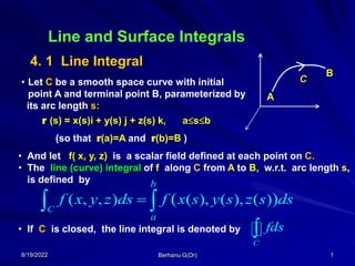
  • 1. 8/19/2022 Berhanu G(Dr) 1 Line and Surface Integrals 4. 1 Line Integral C A B • Let C be a smooth space curve with initial point A and terminal point B, parameterized by its arc length s: • And let f( x, y, z) is a scalar field defined at each point on C. • The line (curve) integral of f along C from A to B, w.r.t. arc length s, is defined by r (s) = x(s)i + y(s) j + z(s) k, asb (so that r(a)=A and r(b)=B ) ( , , ) ( ), ( ), ( ) ( ) C b a f x y z ds f x s y s z s ds    • If C is closed, the line integral is denoted by C fds 
  • 2. 8/19/2022 Berhanu G(Dr) 2 • Example 1: Integrate f(x,y)=xy2 over a circular arc given by r (s) = cos(s) i + sin(s) j , 0 s  /2 • Remark: If a curve C is parameterized by any parameter, say, t : 2 2 / 2 0 2 cos( )sin ( ) 3 C xy ds s s ds      C • Solution: On C, x =cos(s) ; y= sin(s)  f(x,y)=xy2 =cos(s). sin2(s) , on C. Therefore, r (t) = x(t)i + y(t) j + z(t) k, a  t  b, '( ) ds ds dt t dt dt   r then, making change of variable: we get, ( , , ) ( ( )) '( ) C b a f x y z ds f t t dt    r r
  • 3. 8/19/2022 Berhanu G(Dr) 3 • Example 2: Evaluate ( 4 ) C xy z ds   • Solution: C is given by r (t) = A + t (BA) , 0  t  1 = 2t i + t j + (1+2t) k, 0  t  1. So, on C, xy +4z = (2t)t + 4(1+2t) = 2t2 + 8t + 4 and, ds = |r(t) | dt . But |r(t) |= | 2i + j + 2 k | = 3  ds = 3dt Therefore, when C is a straight line segment from point A(0,0, 1) to B = (2, 1,3).
  • 4. 8/19/2022 Berhanu G(Dr) 4 Usually, line integrals that involves a vector field F( x, y, z) that defined on C has the following form: C r(t) A B • Or, representing C by r (t) = x(t)i + y(t) j + z(t) k, a  t  b, . C d  F r where, F( x, y, z) = f1(x,y,z)i + f2 (x,y,z)j + f3 (x,y,z) k, and, dr = dx i + dy j + dz k ( line integral of tangential component of F ) That is, 1 2 3 ( , , ) ( , , ) ( , , ) . C C d f x y z dx f x y z dy f x y z dz      F r '( ) d d dt t dt dt   r r r ( , , ) ( ( )) x y z t  F F r Moreover, on C, We get, ( ( )) '( ) . . b C a d t t dt    F r F r r
  • 5. 8/19/2022 Berhanu G(Dr) 5 • Example 3: Let F(x,y) = (x + y) i + (xy) j . Evaluate when C is: (a) the parabola y=x2 from (1,1) to (4,2) (b) the circle x2+y2 = 1 • Solution: (a) F.dr = (x+y)dx + (xy)dy. But on C, y=x2 , dy=2xdx = (x+x2) dx + (xx2)2x dx = (x + 3x2 2x3) dx, 1  x  4. Hence, (b) C, parametrically, r (t) = cost i + sint j , 0  t  2 r (t) = cost i + sint j ,  r (t) = sint i + cost j , and, F(r(t) ) = (cost + sint) i + (costsint) j . Hence, . C d  F r ( ) ( ) . C C d x y dx x y dy       F r 4 2 3 1 34 3 ( 3 2 ) x x x dx      2 2 0 0 ( ( )) '( ) (cos(2 ) sin(2 )) 0 . . C d t t dt t t dt          F r F r r
  • 6. 8/19/2022 Berhanu G(Dr) 6 • Exercise: 1) Let F(x,y) = x i + x2 j . Evaluate Ans.  4 (1,0) ( 1,0) .d   F r along curve C , from (1,0) to (1,0) in the xy-plane, given by (a) the semi-circle of radius 1 (b) the polygonal path (line segments) shown in the figure below. (1,0) (1,0) (1,1) (0,1) 2) Evaluate where C is the circle x2+y2=4, oriented counterclockwise. C ydx xydy   Ans. (a) 0; (b) ½
  • 7. 8/19/2022 Berhanu G(Dr) 7 At each instant of time t, the particle may be thought as moving in the direction of the tangent to its trajectory, r(t). Hence, F(r(t)).r(t) is the product of force with a direction, and so has the dimension of work. Therefore, the line integral is the work done by the force F in moving the particle from A to B over the path C. ( ( )) '( ) . . b C a d t t dt    F r F r r Remark : Line integrals arise in many context. For example, consider a force F causing a particle to move from point A to point B in space along a smooth curve C whose vector equation r(t) is representing the position of the particle at time t, such that atb, C r(t) A B r (t)
  • 8. 8/19/2022 Berhanu G(Dr) 8 • Suppose C1 and C2 are different curves from point A to B, and let F(x,y,z) be a vector space defined on both curves, 4. 2 Line Integral Independent of Path A B C1 C2 • In a general case, 1 . C d  F r and 2 . C d  F r may not equal. (See, the above exercise. ) • That means, the value of a line integral from point A to B may depend on the curve (path) along which we integrate. (see, the above exercise) • However, for a particular F, if for every curve C1 and C2 that join any point A to B , we say the line integral of F is path independent. 1 2 . . C C d d    F r F r • We will show that line integral of a conservative vector filed F is path independent. Recall: F is conservative if F=f, for some scalar field f (called potential of F)
  • 9. 8/19/2022 Berhanu G(Dr) 9 Theorem: (Fundamental Theorem of Line Integral) Suppose C is a smooth curve from point A(x0,y0,z0) to B(x1,y1,z1) . Let f (x,y,z) be a scalar field, continuously differentiable, on C. Then, A B C Proof: Let r(t), for atb, represents C so that r(a)=A and r(b)=B. ( ) ( ) . C d f B f A f     r • Consequently, the line integral of f is path independent. Hence, the line integral of f along every curve C from point A to B are equal and can be written as '( ) . ( ( ). b C a d t dt f f r t      r r = ( ( ) ( ( ) b b a a d dt f t f t   r r ( ( ) ( ( ) ( ) ( ) f b f a f B f A     r r ( ) ( ) . B A d f B f A f     r
  • 10. 8/19/2022 Berhanu G(Dr) 10 Theorem: (Line Integral of Conservative Vector Fields) The line integral of a conservative vector field is independent of path. In particular, if F is a conservative vector field and C is a curve from point A to B, then where  is a potential of F; i.e., F=  Thus, the line integral of a conservative F over a curve C is the difference of the values of its potential function at the end points of C. ( ) ( ) . . C C d d B A          r r F ( ) ( ) . C d B A      F r Further, if C is a closed curve, then 0 . C d   F r • The proof follows directly from the previous Theorem since,
  • 11. 8/19/2022 Berhanu G(Dr) 11 Example. Evaluate 2 (1, /8) (0,0) 2 cos(2 ) 2 sin(2 ) x y dx x y dy    Solution: This is line integral of F(x,y) = 2xcos(2y) i – 2x2sin(2y) j along certain curve from (0,0) to (1, /8). You can check that F is conservative and its potential function is (x,y) = x2cos(2y). Hence, along any curve in the xy-plane from (0,0) to (1, /8), we get 2 (1, /8) 8 (0,0) 2 2 2 cos(2 ) 2 sin(2 ) (1, ) (0,0) x y dx x y dy         
  • 12. 8/19/2022 Berhanu G(Dr) 12 Exercise. 2 (2,3) (0,1) (2 1) ( 1) xy dx x dy     (a) 2. For the following integrals, C is the ellipse x2 + 4y2 = 16 (5,3,2) (0,0,0) .dr  F (b) , where F(x,y,z) = 3i + zj + (y+2z)k 1. Show that each of the following line integrals are independent of path and evaluate the integrals. . C dr  F (i) , F(x,y,z) = (2xy+z2)i + x2j + (2xz+  cos(z) )k (ii) 2 3 C 3x ydx x dy  
  • 13. 8/19/2022 Berhanu G(Dr) 13 • Green’s Theorem relates certain line integrals over a closed curve with double integrals over plane region enclosed by the curve. 4. 3 Green’s Theorem • Recall the following definition of double integrals: If R ={ (x,y) | a  x b, g1(x) y g2(x) }, y=g1(x) y=g2(x) a b R   2 1 ( ) ( ) R ( , ) ( , ) g x g x b a f x y dxdy x y x f y d d     • OR, if R ={ (x,y) | h1(y) x h2(y) ,c y d },   2 1 ( ) ( ) R ( , ) ( , ) h y h y d c f x y dxdy x y y f x d d     c d R
  • 14. 8/19/2022 Berhanu G(Dr) 14 Theorem: ( Green’s Theorem) 2 1 1 2 R ( , ) ( , ) C f f f x y dx f x y dy dxdy x y                Suppose C is a closed piecewise smooth curve in xy-plane oriented counter clockwise, R is the region enclosed by C; and F(x,y)= f1(x,y) i + f2(x,y) j . Then, R C That is, R . C d dxdy      F r F.k Note: 1. Observe the analogy between Fundamental theorem of Calculus, Fundamental Theorem of line integrals, and Green’s Theorem. 2. Green’s Theorem can be used to evaluate line integrals over a closed piecewise smooth curve in plane.
  • 15. 8/19/2022 Berhanu G(Dr) 15 Example: Use Green’s Theorem to evaluate 3 ( ) ( 1) C x xy dx y dy     where C is the boundary of a square with vertices at the points (1, 0), (2,0), (2, 1) and (1, 1), as shown in the figure below. Solution: f1= x – xy and f2 = y3 +1 (1,0) (2,0) (2,1) (1,1) R C 3 2 1 R ( ) ( 1) C f f x xy dx y dy dxdy x y                  2 2 1 1 1 1 1 0 0 0 3 2 3 = 2 xdx dy x d d dx y y                    
  • 16. 8/19/2022 Berhanu G(Dr) 16 Exercise: Use Green’s Theorem to evaluate where F(x,y)= y i + 5x j and C is the closed curve formed by the three sides of the triangle whose vertices is at (0,0), (2,0) and (0,3), shown in the figure below. . C d  F r 0 2 3 Ans. 12 ( will become 4  area of the triangle ) . C d  F r Reading Assignment: Use of Green’s Theorem to find area of a plane region
  • 17. 8/19/2022 Berhanu G(Dr) 17 • Aim: To evaluate integrals of quantities defined on a surface S. 4. 4 Integrals over Surfaces • Recall: If a surface S is given by f(x,y,z)=c, where c is a constant and f is a differentiable scalar field, then f(x,y,z) is a normal vector to S, at each point (x,y,z) on S; • Like tangent for a curve, normal vector to a surface plays important role to describe the surface (or for various discussion related to the surface). • Also, parametric representation of surfaces is very useful (Since a surface is 2 dimensional, two parameters are required for its parametric representation). 4. 4.1 Surfaces and Normal Vectors
  • 18. 8/19/2022 Berhanu G(Dr) 18 • Examples: 1. A sphere of radius  centered at 0, can be parameterized using: x= cos(u) sin(v) , 0  u 2, and 0  v , y= sin(u) sin(v) , z= cos(v) . • In particular, if every point (x,y,z) on a surface S can be written in terms of two parameters u and v; i.e., if x=x(u,v), y=y(u,v) and z=z(u,v), where a  u b, and c  v d, then S is said to be parametrically represented by r(u,v) = x(u,v) i + y(u,v) j + z(u,v) k, for a  u b & c  v d . u v (x,y,z)  (x,y,0) Thus, r(u,v) =cos(u)sin(v)i +sin(u)sin(v)j + cos(v) k, when 0  u 2, and 0  v .
  • 19. 8/19/2022 Berhanu G(Dr) 19 (x,y,0)  u (x,y,z) z=v 2. The lateral surface of a vertical circular cylinder of radius  and height h can be parameterized using: 3. If S is given by x+y+z=1 over x,y[0,1] , then S can be parameterized using x=u, y=v, z=1uv, where 0  u 1, and 0  v 1. x=cos(u), 0  u 2, y=sin(u), z=v, 0  v h. Thus, r(u,v) =cos(u)i +sin(u)j + v k, when 0  u 2, and 0  vh. Thus, r(u,v) =ui + v j + (1uv) k, when 0  u, v  1.
  • 20. 8/19/2022 Berhanu G(Dr) 20 • Normal vector: If a surface S is given by a differentiable • In general, if S is given by z=f(x,y), for x[a,b] and y[c,d] , then putting x=u and y=v, we can represent S by • r(u,v) = u i + v j + f(u,v) k, where a  u b & c  v d r(u,v) = x(u,v) i + y(u,v) j + z(u,v) k, for a  u b & c  v d , the, a normal vector N to S , called outward normal, is given by N = ru  rv v -constant u -const ru rv N where ru & rv are partial derivatives of r(u,v) w.r.t u & v, respectively In this case, the unit outward normal of S is given by || || u v u v    r r r r n when N = ru  rv  0.
  • 21. 8/19/2022 Berhanu G(Dr) 21 • Definition: A surface S is said to be smooth if it has continuously differentiable parametric representation r(u,v) such that N = ru  rv  0 at every point on S. ( If this definition fails at only some finite points, then S is called piecewise smooth) Surface area: Let S be a smooth surface given parametrically by r(u,v) over a region R = { (u,v) | a u b , c v d } To find the area element A at r(u,v) : Let b = r(u+u,v)  r(u,v) = ruu h = r (u,v+u)  r(u,v) = rvv  A  || b  h || = || ruu  rvv || = || ru rv|| u v || || R u v dudv     r r Some times, dA is used instead of dS So, taking u, v 0, we get dS = || ru rv|| du dv. Hence, the total surface area of S is given by A h r(u,v) b
  • 22. 8/19/2022 Berhanu G(Dr) 22 Exercise: Show that the surface area of a sphere of radius  is 42 . || || R u v dudv     r r To show this: recall that the parametric representation of sphere is r(u,v) =cos(u)sin(v)i +sin(u)sin(v)j + cos(v) k over the region R = { (u,v) | 0  u 2, 0  v  } ; and surface area is given by
  • 23. 8/19/2022 Berhanu G(Dr) 23 4. 4.2 Surface Integral • Let S be a surface of finite area and f(x,y,z) is a function (scalar quantity) defined on S. The total quantity of f on S is given by the following integral, called surface integral of f over S: ( , , ) f x y z d  S S Some times, dS is used instead of dA • To evaluate surface integral, we reduce it to double integral using parametric representation of S. In particular, if S is given by r(u,v) =x(u,v)i + y(u,v)j + z(u,v)k, for a  u b & c  v d, then, f(x,y,z) = f(r(u,v)) over R = {(u,v) | a  u b , c  v d } and dS = || ru rv|| du dv. ( , , ) ( ( , )) || || u v R f x y z d f u v dudv     S S r r r Hence,
  • 24. 8/19/2022 Berhanu G(Dr) 24 Example: Evaluate ( , , ) f x y z d  S S where f(x,y,z) = x+z and S is given by x2+y2=4, 0 z 3 . Solution: Parametric representation of S ( which is cylinder) is: ( , , ) ( ( , )) || || u v R f x y z d f u v dudv     S S r r r r(u,v) = 2cos(u) i + 2sin(u) j + v k , over R= {(u,v) | 0  u 2, 0 v 3} f(r(u,v)) = cos(u) +v; and  ru rv = 2cos(u) i + 2sin(u) j  ||ru rv || =2 ru = 2sin(u) i + 2cos(u) j + o k , rv = 0i + 0 j + 1 k . Hence,   3 3 0 0 0 2 (cos ) 2 9 d u v du v dv v          
  • 25. 8/19/2022 Berhanu G(Dr) 25 ( ( , )) R u v d u v dudv     S F.n S F r . r r || || u v u v    r r r r n Recall: and dS = || ru rv|| du dv. Hence, if a vector field F(x,y) =f1(x,y,z)i + f2(x,y,z)j + f3(x,y,z)k, is defined on a surface S whose parametric representation is r(u,v) =x(u,v)i+y(u,v)j+z(u,v)k over R={(u,v) | a  u b , c  v d }, then, the flux integral through S is given by • Flux integral through a surface S is a surface integral over S in which the integrand is given by F.n : where F is a vector field defined on S and n is the unit outward normal vector to S. d  S F.n S
  • 26. 8/19/2022 Berhanu G(Dr) 26 • Example: Compute the flux integral of F(x,y) = i +xyj through triangular surface S given by x+y+z=1, where 0x, y 1. • Solution: Setting x=u, y=v, z=1uv, S is given by r(u,v) =ui+vj+(1uv)k over R={(u,v) | 0  u, v 1 },  F(r(u,v)) = i +uvj = (1, uv, 0) ru  rv= i + j + k = (1, 1, 1) F(r(u,v))  ru  rv = 1+ uv Hence, N S ( ( , )) R u v d u v dudv     S F.n S F r . r r   1 1 0 0 (1 ) 5 4 uv du dv     
  • 27. 8/19/2022 Berhanu G(Dr) 27 Ans: idea • S is composed of six piecewise smooth surfaces S1, S2, …, S6. Hence, represent each by parametric vector function and compute: • Exercise: Compute the flux integral , of F(x,y,z) = ½ x2 i +yz j +x3yk through the surface (six sides) of the unit cube whose vertices are at (0,0,0), (1, 0, 0), (0,1, 0) and (0, 0,1), as shown in the figure below. d  S F.n S (1,0,0) (0,1,0) (0,0,1) 1 2 6 1 4 d dS dS dS          S S S S F.n S F.n F.n F.n ( The next theorem, Divergence Theorem, provides you with another way of com putting such flux integral)
  • 28. 8/19/2022 Berhanu G(Dr) 28 Theorem (Divergence Theorem): • Let F(x, y, z) be a vector field, S be a piecewise smooth closed surface enclosing a bounded 3D space (volume) V. Then, . V dV d     S F F.n S • Divergence Theorem, also called Gauss Theorem, relates surface(flux) integral across a closed surface S with volume integral over V , where V is the volume (interior space) enclosed by S. • It is 3D analogue of FTC, FTLI and Green’s Theorem) (Here, dV = dx dy dz ) Or (div ) V d dV    S F.n S F In other words, the flux integral of F through a closed surface S is identical to the volume integral of div F taken throughout V. 4. 5 Divergence and Stokes’ Theorems
  • 29. 8/19/2022 Berhanu G(Dr) 29 Solution: div F = .F = x + z V = { (x,y,z) | 0  x, y, z 1 } • Example: Using divergence Theorem, compute the flux integral of F(x,y,z) = ½ x2 i +yz j +x3yk across the closed surface of the unit cube whose vertices are at (0,0,0), (1, 0, 0), (0,1, 0) and (0, 0,1), as shown in the figure below. d  S F.n S (1,0,0) (0,1,0) (0,0,1) V div d dV    S F.n S F     1 0 0 1 0 1 ( 1 ) 4 x dy z dx dz      
  • 30. 8/19/2022 Berhanu G(Dr) 30 Theorem (Stokes’ Theorem): Suppose S is a surface whose boundary is a piecewise smooth closed curve C, with positive orientation, and F(x, y, z) is a vector field defined on S. Then, • The next theorem, called Stokes’ Theorem, is a generalization of Green’s Theorem in 3D. It relates the line integral of vector field F around a closed curve C to the surface integral of curl F. n over surface S whose perimeter (boundary) is C, and n is the unit normal to S. i.e., C S S . C d d      F r F.n S S curl . C d d    F r F.n S
  • 31. 8/19/2022 Berhanu G(Dr) 31 Example: Compute • Solution: To use the Stokes’ Theorem, take the rectangular region whose boundary is the given closed curve C to be the surface S : where F(x,y) = yz i + ½ x2 j + xy2z k and C is the sides of a rectangle on z=3 plane whose vertices are points A(1, 0,3), B(1, 2, 3), C(0, 2, 3) and D(0,0,3), oriented positively. . C d  F r D A B C C S curl . C d d    F r F.n S Here, the unit normal to this S is n = k = (0, 0, 1), and curl F = ( . . ) i + ( . . ) j + ( x+z ) k  curl F. n = x+z = x+3, since z=3 on S, and 0x1, 0y2,   1 2 2 0 0 0 7 2 ( 3 7 ) . C y y x x y d dy x d d             F r
  • 32. 8/19/2022 Berhanu G(Dr) 32 (a) F(x,y) = 2y i + xz3j  zy3 k and C is the circle x2+y2=4 on z=3 plane . (ans. 284 ) (b) F(x,y) = y i + zj + 3y k and C is the intersection of x2+y2+z2=6z and z=x+3 . (ans. ) (c) F(x,y) = y2 i + x2 j  (x+z) k and C is the boundary of the triangle with vertices at (0, 0,0), (1, 0, 0) and (1,1,0). (ans. 1/3 ) Exercise: Using Stokes’ Theorem, evaluate . C d  F r where the vector field F and positively oriented curve C are as given below. 18 2  